Difference between revisions of "UKCA Chemistry and Aerosol vn10.9 Tutorial 10"

Revision as of 10:56, 13 December 2017

UKCA Chemistry and Aerosol Tutorials at vn10.9

What you will learn in this Tutorial

In this tutorial you will learn how to output and process aerosol diagnostics from UKCA.

Python

In this Tutorial you will make extensive use of Python to process the UM output. Instructions as to how to use this are in Tutorial 5.

Example python scripts are provided for each Task, and you should take the time to read through these and understand what they are doing. None of these scripts plot any of the output, so as an extension to these tasks you could try extending the scripts to plot the output from python directly, rather than visualising via Xconv. Further information (and examples) on how Iris plots can be found here:

Task 10.1: Output aerosol diagnostics

TASK 10.1: Output the following aerosol and radiation diagnostics to the UPA output stream. You should make a new time profile (called TRAD) to only output these on radiation timesteps. You will also need to make a new domain profile (called D3DAR) for s02i530 and s02i540, to output these on model levels and pseudo levels.

Hint
Remember to output your aerosol diagnostics on the AOT pseudo levels using the DIAGAOT profile.

STASH Section	STASH Item	STASH Name
1	207	INCOMING SW RAD FLUX (TOA): ALL TSS
1	208	OUTGOING SW RAD FLUX (TOA)
2	205	OUTGOING LW RAD FLUX (TOA)
2	285	MINERAL DUST OPTICAL DEPTH IN RADN.
2	300	AITKEN MODE (SOLUBLE) OPTICAL DEPTH
2	301	ACCUM MODE (SOLUBLE) OPTICAL DEPTH
2	302	COARSE MODE (SOLUBLE) OPTICAL DEPTH
2	303	AITKEN MODE (INSOL) OPTICAL DEPTH
2	304	ACCUM MODE (INSOL) OPTICAL DEPTH
2	305	COARSE MODE (INSOL) OPTICAL DEPTH
2	585	MINERAL DUST ABS. OPICAL DEPTH
2	240	AITKEN (SOLUBLE) ABS OPTICAL DEPTH
2	241	ACCUM (SOLUBLE) ABS OPTICAL DEPTH
2	242	COARSE (SOLUBLE) ABS OPTICAL DEPTH
2	243	AITKEN (INSOL) ABS OPTICAL DEPTH
2	244	ACCUM (INSOL) ABS OPTICAL DEPTH
2	245	COARSE (INSOL) ABS OPTICAL DEPTH
2	530	UKCA 3D AEROSOL EXTINCTION
2	540	CLASSIC 3D AEROSOL EXTINCTION

Radiation Timesteps

The number of shortwave radiation timesteps per day is given by i_sw_radstep_perday_prog, found in um $\rightarrow$ namelist $\rightarrow$ UM Science Settings $\rightarrow$ Section 01 - 02 Radiation $\rightarrow$ Shortwave. The equivalent for longwave is i_lw_radstep_perday_prog, found in um $\rightarrow$ namelist $\rightarrow$ UM Science Settings $\rightarrow$ Section 01 - 02 Radiation $\rightarrow$ Longwave.

In the UKCA training suite, both of these are set to 16, i.e. a call every 90 minutes. This value is very configuration dependent - sometimes radiation is called every hour (24), sometimes every 3 hours (8) etc. You should check the settings in your suite if you need to consider any of the radiation diagnostics.

Making new STASH profiles

While we have covered outputting and creating new diagnostics in Tutorial 3, Tutorial 4, Tutorial 5, and Tutorial 9, you were only making use of existing profiles. Here you will learn how to make new time, domain, and usage profiles.

Time profiles

The new time panel in Rose.

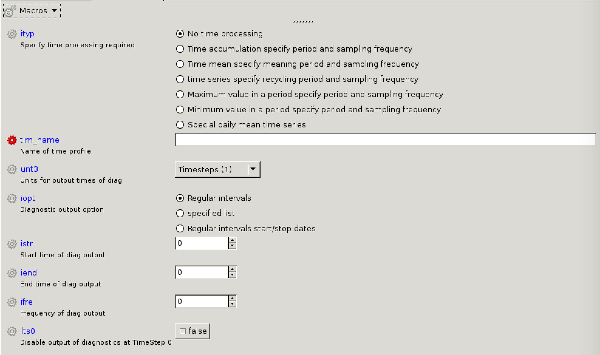
To make a new time profile, go to: um $\rightarrow$ namelist $\rightarrow$ Model Input and Output $\rightarrow$ STASH Requests and Profiles $\rightarrow$ Time Profiles. This contains a list of existing time profiles, with names like t3hmn_039ecafe etc.

To make a new time profile, you should:

Right-click anywhere on the list and click the blue plus symbol named new section
This will make a new blank line (usually labelled 1, the next 2 etc.) with a red X next to it.
Right-click this new line and click View namelist.
Fill-in the values as required for what you want to do.

Example: Output on Radiation Timesteps

You will have discovered that there are 16 radiation timesteps per day, but to work out how to output diagnostics you need to know many model timesteps per day there are. This can be found at: um $\rightarrow$ namelist $\rightarrow$ Top Level Model Control $\rightarrow$ Model Domain and Timestep. The number is given by the variable steps_per_periodim, which is defined as the number of steps per period given (in seconds) by secs_per_periodim. For one day, this value is 86400.

In the UKCA training suite, secs_per_periodim=86400, and steps_per_periodim=48. This means that there are 48 timesteps per day, i.e. each timestep is 30 minutes.

We can combine this with the number of radiation timesteps per day (16), to calculate that radiation is called every third model timestep (48/16 = 3) in this configuration. We can now fill-in the values in the new time profile accordingly, e.g.

ityp: No time processing
tim_name: e.g. TRAD
unt3: Timesteps (1)
iopt: Regular intervals
istr: 1 (i.e. start on first timestep)
iend: -1 (i.e. never stop outputting)
ifre: 3 (i.e. output every third timestep)

We need to start at timestep 1, as radiation is called on the first timestep, and then called every third model timestep after that. In contrast, the UKCA Newton-Raphson chemical solver is first called on the first hour, and then every hour after that. For the UKCA training suite this would mean that istr=2 and ifre=2.

Domain profiles

The new domain panel in Rose.

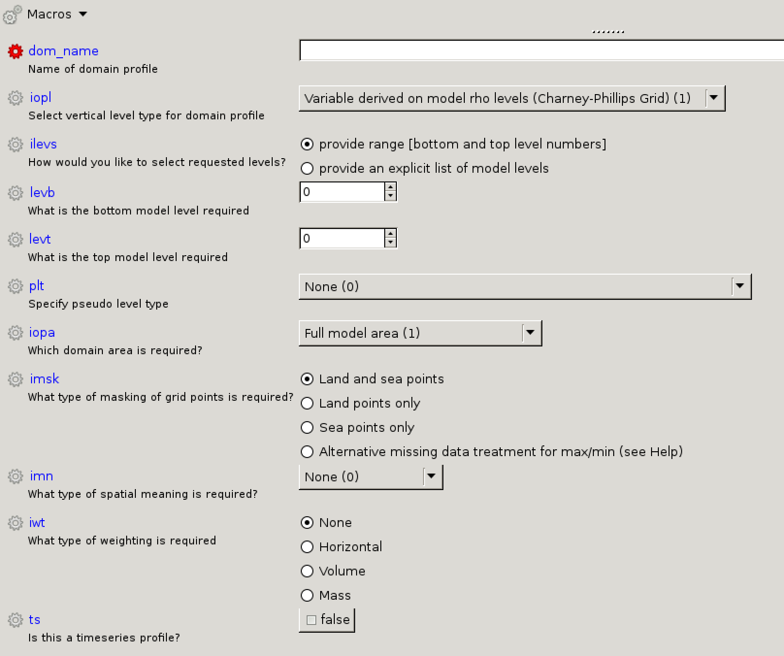
To make a new time profile, go to: um $\rightarrow$ namelist $\rightarrow$ Model Input and Output $\rightarrow$ STASH Requests and Profiles $\rightarrow$ Domain Profiles. This contains a list of existing domain profiles, with names like dallth_1e2e730d etc.

To make a new domain profile, you should:

Right-click anywhere on the list and click the blue plus symbol (+) named new section
This will make a new blank line (usually labelled 1, the next 2 etc.) with a red X next to it.
Right-click this new line and click View namelist.
Fill-in the values as required for what you want to do.

Example: Output AOT pseudo levels on all model theta levels

Aerosol diagnostics are defined on a series of 6 pseudo levels, corresponding to 0.38, 0.44, 0.55, 0.67, 0.87, and 1.02 microns. You will therefore need to output on your data on all of these. For some diagnostics, such as AOD, these are defined on a single level, but others, such as extinction, are a 3D field over the whole atmosphere. Therefore, to output the 3D aerosol extinction we need to make a new profile over all model (theta grid) levels, and all 6 pseudo levels.

We can now fill-in the values in the new domain profile accordingly, e.g.

dom_name: e.g. D3DAR
iopl: Variable derived on model theta levels (Charney-Phillips Grid) (2)
ilevs: provide range [bottom and top level numbers]
ilevb: 1 (i.e. 20m level)
ilevt: 85 (i.e. highest level)
plt: Radiation bands for calculating aerosol optical depth (4)

This will then insert a new option below (pslist) to allow you to specify the bands you require.

pslist: press the blue plus symbol (+) 5 times, and enter the numbers 1 to 6 in each of the boxes to output all AOT pseudo levels.
iopa: Full model area (1)
imsk: Land and sea points
imn: None (0)
iwt: None
ts: false

Usage profiles

The new usage panel in Rose.

Making new usage profiles is not as straight-forward as for time and domain profiles, as these are used to output diagnostics to different output files (and possibly to climate mean files). To see what output streams are available, go to: um $\rightarrow$ namelist $\rightarrow$ Model Input and Output $\rightarrow$ Model Output Streams. In the UKCA training suite, only pp0 is active.

To look at climate meaning, go to: um $\rightarrow$ namelist $\rightarrow$ Model Input and Output $\rightarrow$ Dumping and Meaning. This is controlled by the logical l_meaning_sequence, which in the UKCA training suite is set to false (i.e. no climate meaning). If this is set to true then various settings will need to be chosen, such as the reference time, the frequency of files, and which files to output.

To make a new usage profile, go to: um $\rightarrow$ namelist $\rightarrow$ Model Input and Output $\rightarrow$ STASH Requests and Profiles $\rightarrow$ Usage Profiles. This contains a list of existing domain profiles, with names like upa_ffb3f00b etc. If you look at the upa namelist (by right-clicking on it and clicking view namelist) you can see that this corresponds with the pp0 output stream.

It is also possible to write diagnostics to a tag, which can then be read by other parts of the code. This is how UKCA couples to the UM, via tag=98. This can be seen in the upukca usage profile.

When you take a copy of an existing configuration it is unlikely that you will need to make any changes to any (or make new) usage profiles. However, if you do want to make a new usage profile, you should:

Right-click anywhere on the list and click the blue plus symbol named new section
This will make a new blank line (usually labelled 1, the next 2 etc.) with a red X next to it.
Right-click this new line and click View namelist.
Fill-in the values as required for what you want to do.

Note that if you are making a new usage profile that is not associated with a tag, you may also need to make changes to the output streams. This could be quite involved.

Using your new profiles

Once you have made your new profiles you should then use them in the usual way, as covered in Tutorial 3.

Solution to Task 10.1

You were given the task

Output the following aerosol and radiation diagnostics to the UPA output stream. You should make a new time profile (called TRAD) to only output these on radiation timesteps. You will also need to make a new domain profile (called D3DAR) for s02i530 and s02i540, to output these on model levels and pseudo levels.

STASH Section	STASH Item	STASH Name
1	207	INCOMING SW RAD FLUX (TOA): ALL TSS
1	208	OUTGOING SW RAD FLUX (TOA)
2	205	OUTGOING LW RAD FLUX (TOA)
2	285	MINERAL DUST OPTICAL DEPTH IN RADN.
2	300	AITKEN MODE (SOLUBLE) OPTICAL DEPTH
2	301	ACCUM MODE (SOLUBLE) OPTICAL DEPTH
2	302	COARSE MODE (SOLUBLE) OPTICAL DEPTH
2	303	AITKEN MODE (INSOL) OPTICAL DEPTH
2	304	ACCUM MODE (INSOL) OPTICAL DEPTH
2	305	COARSE MODE (INSOL) OPTICAL DEPTH
2	585	MINERAL DUST ABS. OPICAL DEPTH
2	240	AITKEN (SOLUBLE) ABS OPTICAL DEPTH
2	241	ACCUM (SOLUBLE) ABS OPTICAL DEPTH
2	242	COARSE (SOLUBLE) ABS OPTICAL DEPTH
2	243	AITKEN (INSOL) ABS OPTICAL DEPTH
2	244	ACCUM (INSOL) ABS OPTICAL DEPTH
2	245	COARSE (INSOL) ABS OPTICAL DEPTH
2	530	UKCA 3D AEROSOL EXTINCTION
2	540	CLASSIC 3D AEROSOL EXTINCTION

and were given the hint

Remember to output your aerosol diagnostics on the AOT pseudo levels using the DIAGAOT profile.

For a working Rose suite that has completed this task, please see

ARCHER: u-as292@62651
vm: u-as297@62631

The specific Rose changes made are:

ARCHER:

Index: app/um/rose-app.conf
===================================================================
--- app/um/rose-app.conf       (revision 60289)
+++ app/um/rose-app.conf       (revision 62651)
@@ -2744,6 +2744,40 @@
 precip_segment_size=32
 ukca_mode_seg_size=4
 
+[namelist:umstash_domain(d3dar_72578706)]
+dom_name='D3DAR'
+!!iest=0
+ilevs=1
+imn=0
+imsk=1
+!!inth=0
+iopa=1
+iopl=2
+!!isth=0
+!!iwst=0
+iwt=0
+!!l_spml_ts=.false.
+levb=01
+!!levlst=0
+levt=85
+plt=4
+pslist=1,2,3,4,5,6
+!!rlevlst=0
+!!spml_bot=0
+!!spml_ew=0
+!!spml_ns=0
+!!spml_top=0
+!!tblim=0
+!!tblimr=0
+!!telim=0
+!!tnlim=0
+ts=.false.
+!!tslim=0
+!!tsnum=0
+!!ttlim=0
+!!ttlimr=0
+!!twlim=0
+
 [namelist:umstash_domain(dallrh_0496a967)]
 dom_name='DALLRH'
 !!iest=0
@@ -3025,6 +3059,22 @@
 tim_name='TALLTS'
 use_name='UPUKCA'
 
+[namelist:umstash_streq(01207_ed72c304)]
+dom_name='DIAG'
+isec=1
+item=207
+package=
+tim_name='TRAD'
+use_name='UPA'
+
+[namelist:umstash_streq(01208_83140cd8)]
+dom_name='DIAG'
+isec=1
+item=208
+package=
+tim_name='TRAD'
+use_name='UPA'
+
 [namelist:umstash_streq(01235_3511dd9f)]
 dom_name='DIAG'
 isec=1
@@ -3033,14 +3083,142 @@
 tim_name='TALLTS'
 use_name='UPUKCA'
 
-[namelist:umstash_streq(02301_0f7c5f4a)]
+[namelist:umstash_streq(02205_357bf644)]
+dom_name='DIAG'
+isec=2
+item=205
+package=
+tim_name='TRAD'
+use_name='UPA'
+
+[namelist:umstash_streq(02240_d97aaab7)]
 dom_name='DIAGAOT'
 isec=2
+item=240
+package=' '
+tim_name='TRAD'
+use_name='UPA'
+
+[namelist:umstash_streq(02241_8cda3169)]
+dom_name='DIAGAOT'
+isec=2
+item=241
+package=' '
+tim_name='TRAD'
+use_name='UPA'
+
+[namelist:umstash_streq(02242_91e371db)]
+dom_name='DIAGAOT'
+isec=2
+item=242
+package=' '
+tim_name='TRAD'
+use_name='UPA'
+
+[namelist:umstash_streq(02243_21bc5f11)]
+dom_name='DIAGAOT'
+isec=2
+item=243
+package=' '
+tim_name='TRAD'
+use_name='UPA'
+
+[namelist:umstash_streq(02244_32fe0790)]
+dom_name='DIAGAOT'
+isec=2
+item=244
+package=' '
+tim_name='TRAD'
+use_name='UPA'
+
+[namelist:umstash_streq(02245_da00b6ef)]
+dom_name='DIAGAOT'
+isec=2
+item=245
+package=' '
+tim_name='TRAD'
+use_name='UPA'
+
+[namelist:umstash_streq(02285_1d9800f0)]
+dom_name='DIAGAOT'
+isec=2
+item=285
+package=' '
+tim_name='TRAD'
+use_name='UPA'
+
+[namelist:umstash_streq(02300_8b9907b5)]
+dom_name='DIAGAOT'
+isec=2
+item=300
+package=' '
+tim_name='TRAD'
+use_name='UPA'
+
+[namelist:umstash_streq(02301_b8711d23)]
+dom_name='DIAGAOT'
+isec=2
 item=301
-package='UKCA Testing'
-tim_name='T3HMN'
+package=' '
+tim_name='TRAD'
 use_name='UPA'
 
+[namelist:umstash_streq(02302_420d0ec7)]
+dom_name='DIAGAOT'
+isec=2
+item=302
+package=' '
+tim_name='TRAD'
+use_name='UPA'
+
+[namelist:umstash_streq(02303_ad5c3af4)]
+dom_name='DIAGAOT'
+isec=2
+item=303
+package=' '
+tim_name='TRAD'
+use_name='UPA'
+
+[namelist:umstash_streq(02304_8c1869b6)]
+dom_name='DIAGAOT'
+isec=2
+item=304
+package=' '
+tim_name='TRAD'
+use_name='UPA'
+
+[namelist:umstash_streq(02305_9ecd020a)]
+dom_name='DIAGAOT'
+isec=2
+item=305
+package=' '
+tim_name='TRAD'
+use_name='UPA'
+
+[namelist:umstash_streq(02530_7a218781)]
+dom_name='D3DAR'
+isec=2
+item=530
+package=' '
+tim_name='TRAD'
+use_name='UPA'
+
+[namelist:umstash_streq(02540_56484a28)]
+dom_name='D3DAR'
+isec=2
+item=540
+package=' '
+tim_name='TRAD'
+use_name='UPA'
+
+[namelist:umstash_streq(02585_38287367)]
+dom_name='DIAGAOT'
+isec=2
+item=585
+package=' '
+tim_name='TRAD'
+use_name='UPA'
+
 [namelist:umstash_streq(03025_c8768f77)]
 dom_name='DIAG'
 isec=3
@@ -3551,6 +3729,25 @@
 !!unt2=2
 unt3=1
 
+[namelist:umstash_time(trad_4c3a45a7)]
+!!iedt=0
+iend=-1
+ifre=3
+!!intv=0
+!!ioff=0
+iopt=1
+!!isam=0
+!!isdt=0
+!!iser=0
+istr=1
+!!itimes=0
+ityp=1
+!!lts0=.false.
+tim_name='TRAD'
+!!unt1=2
+!!unt2=2
+unt3=1
+
 [namelist:umstash_use(upa_ffb3f00b)]
 file_id='pp0'
 locn=3

These differences can be found in the file /home/ukca/Tutorial/vn10.9/worked_solutions/Task10.1/Task10.1_rose.patch on PUMA.

vm:

Index: app/um/rose-app.conf
===================================================================
--- app/um/rose-app.conf       (revision 60286)
+++ app/um/rose-app.conf       (revision 62631)
@@ -2849,6 +2849,40 @@
 !!ttlimr=0.0
 !!twlim=0
 
+[namelist:umstash_domain(d3dar_72578706)]
+dom_name='D3DAR'
+!!iest=0
+ilevs=1
+imn=0
+imsk=1
+!!inth=0
+iopa=1
+iopl=2
+!!isth=0
+!!iwst=0
+iwt=0
+!!l_spml_ts=.false.
+levb=01
+!!levlst=0
+levt=85
+plt=4
+pslist=1,2,3,4,5,6
+!!rlevlst=0
+!!spml_bot=0
+!!spml_ew=0
+!!spml_ns=0
+!!spml_top=0
+!!tblim=0
+!!tblimr=0
+!!telim=0
+!!tnlim=0
+ts=.false.
+!!tslim=0
+!!tsnum=0
+!!ttlim=0
+!!ttlimr=0
+!!twlim=0
+
 [namelist:umstash_domain(dallrh_0496a967)]
 dom_name='DALLRH'
 !!iest=0
@@ -3617,6 +3651,22 @@
 tim_name='TALLTS'
 use_name='UPUKCA'
 
+[namelist:umstash_streq(01207_ed72c304)]
+dom_name='DIAG'
+isec=1
+item=207
+package=
+tim_name='TRAD'
+use_name='UPA'
+
+[namelist:umstash_streq(01208_83140cd8)]
+dom_name='DIAG'
+isec=1
+item=208
+package=
+tim_name='TRAD'
+use_name='UPA'
+
 [namelist:umstash_streq(01235_3511dd9f)]
 dom_name='DIAG'
 isec=1
@@ -3625,14 +3675,142 @@
 tim_name='TALLTS'
 use_name='UPUKCA'
 
-[namelist:umstash_streq(02301_0f7c5f4a)]
+[namelist:umstash_streq(02205_357bf644)]
+dom_name='DIAG'
+isec=2
+item=205
+package=
+tim_name='TRAD'
+use_name='UPA'
+
+[namelist:umstash_streq(02240_d97aaab7)]
 dom_name='DIAGAOT'
 isec=2
+item=240
+package=' '
+tim_name='TRAD'
+use_name='UPA'
+
+[namelist:umstash_streq(02241_8cda3169)]
+dom_name='DIAGAOT'
+isec=2
+item=241
+package=' '
+tim_name='TRAD'
+use_name='UPA'
+
+[namelist:umstash_streq(02242_91e371db)]
+dom_name='DIAGAOT'
+isec=2
+item=242
+package=' '
+tim_name='TRAD'
+use_name='UPA'
+
+[namelist:umstash_streq(02243_21bc5f11)]
+dom_name='DIAGAOT'
+isec=2
+item=243
+package=' '
+tim_name='TRAD'
+use_name='UPA'
+
+[namelist:umstash_streq(02244_32fe0790)]
+dom_name='DIAGAOT'
+isec=2
+item=244
+package=' '
+tim_name='TRAD'
+use_name='UPA'
+
+[namelist:umstash_streq(02245_da00b6ef)]
+dom_name='DIAGAOT'
+isec=2
+item=245
+package=' '
+tim_name='TRAD'
+use_name='UPA'
+
+[namelist:umstash_streq(02285_1d9800f0)]
+dom_name='DIAGAOT'
+isec=2
+item=285
+package=' '
+tim_name='TRAD'
+use_name='UPA'
+
+[namelist:umstash_streq(02300_8b9907b5)]
+dom_name='DIAGAOT'
+isec=2
+item=300
+package=' '
+tim_name='TRAD'
+use_name='UPA'
+
+[namelist:umstash_streq(02301_b8711d23)]
+dom_name='DIAGAOT'
+isec=2
 item=301
-package='UKCA Testing'
-tim_name='T3HMN'
+package=' '
+tim_name='TRAD'
 use_name='UPA'
 
+[namelist:umstash_streq(02302_420d0ec7)]
+dom_name='DIAGAOT'
+isec=2
+item=302
+package=' '
+tim_name='TRAD'
+use_name='UPA'
+
+[namelist:umstash_streq(02303_ad5c3af4)]
+dom_name='DIAGAOT'
+isec=2
+item=303
+package=' '
+tim_name='TRAD'
+use_name='UPA'
+
+[namelist:umstash_streq(02304_8c1869b6)]
+dom_name='DIAGAOT'
+isec=2
+item=304
+package=' '
+tim_name='TRAD'
+use_name='UPA'
+
+[namelist:umstash_streq(02305_9ecd020a)]
+dom_name='DIAGAOT'
+isec=2
+item=305
+package=' '
+tim_name='TRAD'
+use_name='UPA'
+
+[namelist:umstash_streq(02530_7a218781)]
+dom_name='D3DAR'
+isec=2
+item=530
+package=' '
+tim_name='TRAD'
+use_name='UPA'
+
+[namelist:umstash_streq(02540_56484a28)]
+dom_name='D3DAR'
+isec=2
+item=540
+package=' '
+tim_name='TRAD'
+use_name='UPA'
+
+[namelist:umstash_streq(02585_38287367)]
+dom_name='DIAGAOT'
+isec=2
+item=585
+package=' '
+tim_name='TRAD'
+use_name='UPA'
+
 [namelist:umstash_streq(03025_c8768f77)]
 dom_name='DIAG'
 isec=3
@@ -4504,6 +4682,25 @@
 unt2=2
 unt3=4
 
+[namelist:umstash_time(trad_4c3a45a7)]
+!!iedt=0
+iend=-1
+ifre=3
+!!intv=0
+!!ioff=0
+iopt=1
+!!isam=0
+!!isdt=0
+!!iser=0
+istr=1
+!!itimes=0
+ityp=1
+!!lts0=.false.
+tim_name='TRAD'
+!!unt1=2
+!!unt2=2
+unt3=1
+
 [namelist:umstash_time(traddm_fa7c24ce)]
 !!iedt=0
 iend=-1

If you open the .pa file in Xconv, you should see the following additional fields:

0    : 96    72    1     2     field200: INCOMING SW RAD FLUX (TOA): ALL TSS 
1    : 96    72    1     2     field201: OUTGOING SW RAD FLUX (TOA)          
2    : 96    72    1     2     olr: OUTGOING LW RAD FLUX (TOA)
3    : 96    72    6     2     unspecified: Stash code = 2240      
4    : 96    72    6     2     unspecified: Stash code = 2241      
5    : 96    72    6     2     unspecified: Stash code = 2242      
6    : 96    72    6     2     unspecified: Stash code = 2243      
7    : 96    72    6     2     unspecified: Stash code = 2244      
8    : 96    72    6     2     unspecified: Stash code = 2245      
9    : 96    72    6     2     unspecified: MINERAL DUST OPTICAL DEPTH IN RADN. 
10   : 96    72    6     2     unspecified: AITKEN MODE (SOLUBLE) OPTICAL DEPTH 
11   : 96    72    6     2     unspecified: ACCUM MODE (SOLUBLE) OPTICAL DEPTH  
12   : 96    72    6     2     unspecified: COARSE MODE (SOLUBLE) OPTICAL DEPTH 
13   : 96    72    6     2     unspecified: AITKEN MODE (INSOL) OPTICAL DEPTH   
14   : 96    72    6     2     unspecified: ACCUM MODE (INSOL) OPTICAL DEPTH    
15   : 96    72    6     2     unspecified: COARSE MODE (INSOL) OPTICAL DEPTH   
16   : 96    72    38    2     unspecified: Stash code = 2530
17   : 96    72    38    2     unspecified: Stash code = 2530
18   : 96    72    38    2     unspecified: Stash code = 2530
19   : 96    72    38    2     unspecified: Stash code = 2530
20   : 96    72    38    2     unspecified: Stash code = 2530
21   : 96    72    38    2     unspecified: Stash code = 2530
22   : 96    72    38    2     unspecified: Stash code = 2540
23   : 96    72    38    2     unspecified: Stash code = 2540
24   : 96    72    38    2     unspecified: Stash code = 2540
25   : 96    72    38    2     unspecified: Stash code = 2540
26   : 96    72    38    2     unspecified: Stash code = 2540
27   : 96    72    38    2     unspecified: Stash code = 2540
28   : 96    72    6     2     unspecified: Stash code = 2585

Sample output from this task can be found at /work/n02/n02/ukca/Tutorial/vn10.9/sample_output/Task10.1/atmosa.pa19810901_00 on ARCHER.

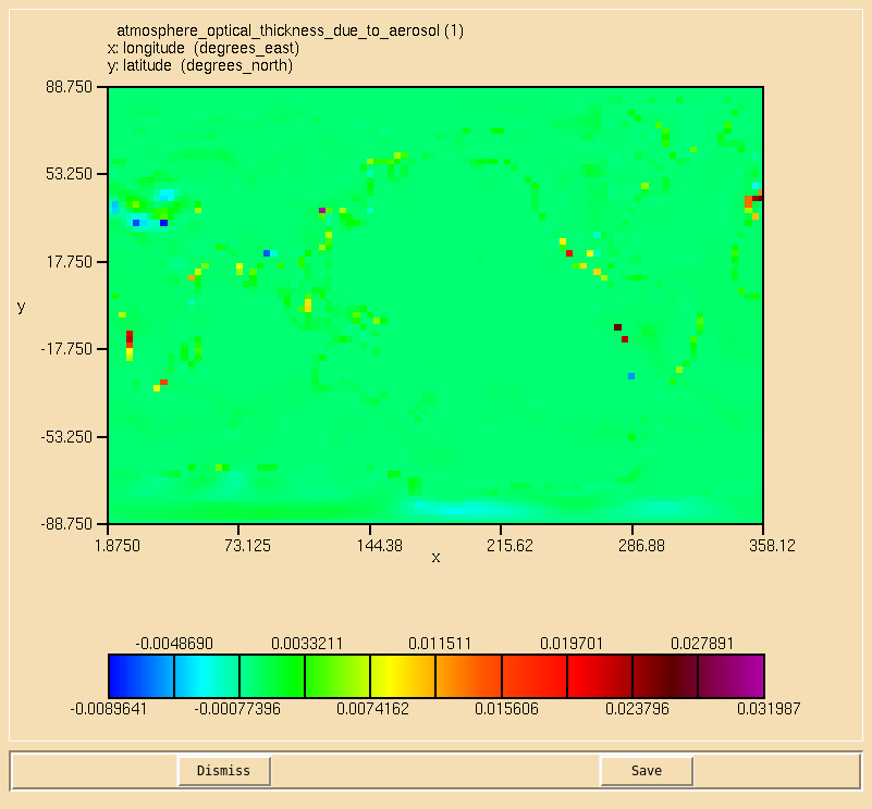
Task 10.2: Calculate aerosol optical depth

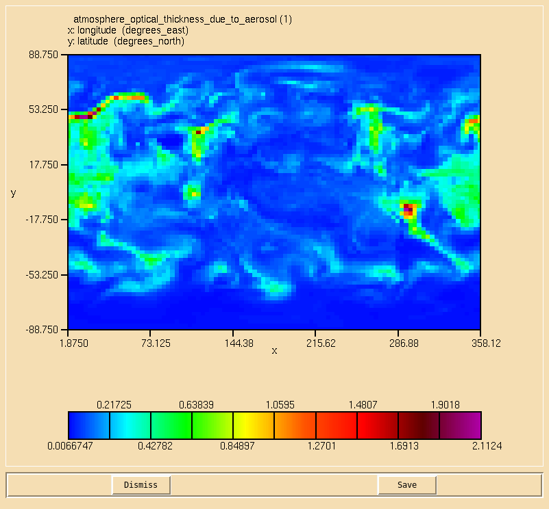
TASK 10.2: Calculate the aerosol optical depth at 0.55 microns on the second radiation timestep.

Hint
The UM calculate optical depth diagnostics on 6 pseudo levels corresponding to 0.38, 0.44, 0.55, 0.67, 0.87, and 1.02 microns, therefore 0.55 microns is pseudo level 3.

Note: You will need to use the CLASSIC mineral dust optical depth diagnostic, as the configuration used in these tutorials does not use modal dust. Likewise, the insoluble accumulation and coarse mode diagnostics will be zero as these modes are not used in the configuration used here.

Python script

To calculate the total aerosol optical depth at 0.55 microns, you should sum up the contribution from the different aerosol components.

On ARCHER, an example python script to do this has been provided at /work/n02/n02/ukca/Tutorial/vn10.9/sample_output/Task10.2/write_AOD.py:

#!/usr/bin/env python

# This file is part of the UKCA Tutorials:
#  http://www.ukca.ac.uk/wiki/index.php/UKCA_Chemistry_and_Aerosol_Tutorials_at_vn10.9

# Copyright (C) 2017  University of Cambridge

# This is free software: you can redistribute it and/or modify it under the
# terms of the GNU Lesser General Public License as published by the Free
# Software Foundation, either version 3 of the License, or (at your option)
# any later version.

# It is distributed in the hope that it will be useful, but WITHOUT ANY
# WARRANTY; without even the implied warranty of MERCHANTABILITY or FITNESS FOR
# A PARTICULAR PURPOSE.  See the GNU Lesser General Public License for more
# details.

# You find a copy of the GNU Lesser General Public License at <http://www.gnu.org/licenses/>.

# Written by N. Luke Abraham 2017-12-11 <nla27@cam.ac.uk> 

# preamble
import iris
import iris.time

fname='/work/n02/n02/ukca/Tutorial/vn10.9/sample_output/Task10.1/atmosa.pa19810901_00'

# constraint on time to get 2nd radiation timestep
tconstr=iris.Constraint(time=lambda cell: cell.point.hour == 2)

# load all AOD components at 0.55 micron
# must use this way of loading to account for constraint on time
with iris.FUTURE.context(cell_datetime_objects=True):
    aod=iris.load(fname,[
        iris.Constraint(pseudo_level=3) & iris.AttributeConstraint(STASH='m01s02i285') & tconstr,
       iris.Constraint(pseudo_level=3) & iris.AttributeConstraint(STASH='m01s02i300') & tconstr,
       iris.Constraint(pseudo_level=3) & iris.AttributeConstraint(STASH='m01s02i301') & tconstr,
       iris.Constraint(pseudo_level=3) & iris.AttributeConstraint(STASH='m01s02i302') & tconstr,
       iris.Constraint(pseudo_level=3) & iris.AttributeConstraint(STASH='m01s02i303') & tconstr,
       iris.Constraint(pseudo_level=3) & iris.AttributeConstraint(STASH='m01s02i304') & tconstr,
       iris.Constraint(pseudo_level=3) & iris.AttributeConstraint(STASH='m01s02i305') & tconstr])

# make cube to store total AOD
aodsum=aod[0].copy()

# add-up components
aodsum.data=aod[0].data+aod[1].data+aod[2].data+aod[3].data+aod[4].data+aod[5].data+aod[6].data

# rename
aodsum.rename('atmosphere_optical_thickness_due_to_aerosol')

# remove unlimited dimension when writing to netCDF
iris.FUTURE.netcdf_no_unlimited=True

# output to netCDF
iris.save(aodsum,'Task102_AOD.nc',netcdf_format='NETCDF3_CLASSIC')

Solution to Task 10.2

0.55 micron AOD calculated from the component aerosol AOD diagnostics.

You were asked to

Calculate the aerosol optical depth at 0.55 microns on the second radiation timestep.

and were given the hint

The UM calculate optical depth diagnostics on 6 pseudo levels corresponding to 0.38, 0.44, 0.55, 0.67, 0.87, and 1.02 microns, therefore 0.55 microns is pseudo level 3.

You should make use of the python script provided to do this.

Sample output from this task can be found in the /work/n02/n02/ukca/Tutorial/vn10.9/sample_output/Task10.2/ directory on ARCHER, containing the following:

Task102_AOD.nc
write_AOD.py

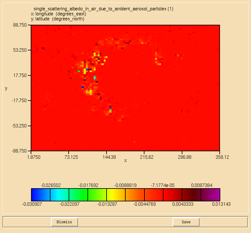
Task 10.3: Calculate the single-scattering albedo

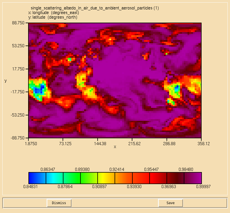
TASK 10.3: Calculate the single-scattering albedo at 0.55 microns on the second radiation timestep, defined as:

$1-\left({\frac {\textrm {Absorption\ Aerosol\ Optical\ Depth}}{\textrm {Aerosol\ Optical\ Depth}}}\right)$

Python script

To calculate the single-scattering albedo at 0.55 microns, you should sum up the contribution to AAOD and AOD from the different aerosol components.

On ARCHER, an example python script to do this has been provided at /work/n02/n02/ukca/Tutorial/vn10.9/sample_output/Task10.3/write_SSA.py:

#!/usr/bin/env python

# This file is part of the UKCA Tutorials:
#  http://www.ukca.ac.uk/wiki/index.php/UKCA_Chemistry_and_Aerosol_Tutorials_at_vn10.9

# Copyright (C) 2017  University of Cambridge

# This is free software: you can redistribute it and/or modify it under the
# terms of the GNU Lesser General Public License as published by the Free
# Software Foundation, either version 3 of the License, or (at your option)
# any later version.

# It is distributed in the hope that it will be useful, but WITHOUT ANY
# WARRANTY; without even the implied warranty of MERCHANTABILITY or FITNESS FOR
# A PARTICULAR PURPOSE.  See the GNU Lesser General Public License for more
# details.

# You find a copy of the GNU Lesser General Public License at <http://www.gnu.org/licenses/>.

# Written by N. Luke Abraham 2017-12-11 <nla27@cam.ac.uk> 

# preamble
import iris
import iris.time

fname='/work/n02/n02/ukca/Tutorial/vn10.9/sample_output/Task10.1/atmosa.pa19810901_00'

# constraint on time to get 2nd radiation timestep
tconstr=iris.Constraint(time=lambda cell: cell.point.hour == 2)

# load all AOD & AAOD components at 0.55 micron
# must use this way of loading to account for constraint on time
with iris.FUTURE.context(cell_datetime_objects=True):
    aod=iris.load(fname,[
        iris.Constraint(pseudo_level=3) & iris.AttributeConstraint(STASH='m01s02i285') & tconstr,
       iris.Constraint(pseudo_level=3) & iris.AttributeConstraint(STASH='m01s02i300') & tconstr,
       iris.Constraint(pseudo_level=3) & iris.AttributeConstraint(STASH='m01s02i301') & tconstr,
       iris.Constraint(pseudo_level=3) & iris.AttributeConstraint(STASH='m01s02i302') & tconstr,
       iris.Constraint(pseudo_level=3) & iris.AttributeConstraint(STASH='m01s02i303') & tconstr,
       iris.Constraint(pseudo_level=3) & iris.AttributeConstraint(STASH='m01s02i304') & tconstr,
       iris.Constraint(pseudo_level=3) & iris.AttributeConstraint(STASH='m01s02i305') & tconstr])
    aaod=iris.load(fname,[
         iris.Constraint(pseudo_level=3) & iris.AttributeConstraint(STASH='m01s02i585') & tconstr,
        iris.Constraint(pseudo_level=3) & iris.AttributeConstraint(STASH='m01s02i240') & tconstr,
        iris.Constraint(pseudo_level=3) & iris.AttributeConstraint(STASH='m01s02i241') & tconstr,
        iris.Constraint(pseudo_level=3) & iris.AttributeConstraint(STASH='m01s02i242') & tconstr,
        iris.Constraint(pseudo_level=3) & iris.AttributeConstraint(STASH='m01s02i243') & tconstr,
        iris.Constraint(pseudo_level=3) & iris.AttributeConstraint(STASH='m01s02i244') & tconstr,
        iris.Constraint(pseudo_level=3) & iris.AttributeConstraint(STASH='m01s02i245') & tconstr])

# make cube to store total AOD
aodsum=aod[0].copy()
# add-up components
aodsum.data=aod[0].data+aod[1].data+aod[2].data+aod[3].data+aod[4].data+aod[5].data+aod[6].data

# make cube to store total AAOD
aaodsum=aaod[0].copy()
# add-up components
aaodsum.data=aaod[0].data+aaod[1].data+aaod[2].data+aaod[3].data+aaod[4].data+aaod[5].data+aaod[6].data

# calculate single-scattering albedo
ssa=aodsum.copy()
ssa.data = 1.0 - (aaodsum.data/aodsum.data)

# rename
ssa.rename('single_scattering_albedo_in_air_due_to_ambient_aerosol_particles')

# remove unlimited dimension when writing to netCDF
iris.FUTURE.netcdf_no_unlimited=True

# output to netCDF
iris.save(ssa,'Task103_SSA.nc',netcdf_format='NETCDF3_CLASSIC')

Solution to Task 10.3

0.55 micron single-scattering albedo.

You were asked to

Calculate the single-scattering albedo at 0.55 microns on the second radiation timestep, defined as:

$1-\left({\frac {\textrm {Absorption\ Aerosol\ Optical\ Depth}}{\textrm {Aerosol\ Optical\ Depth}}}\right)$

You should use the python script provided to do this.

Sample output from this task can be found in the /work/n02/n02/ukca/Tutorial/vn10.9/sample_output/Task10.3/ directory on ARCHER, containing the following:

Task103_SSA.nc
write_SSA.py

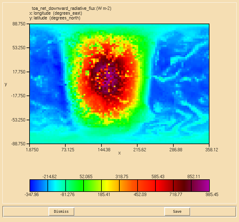
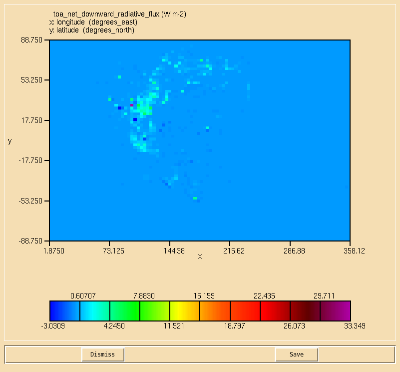
Task 10.4: Calculate the top of the atmosphere net downward radiative flux

TASK 10.4: Calculate the net downward top of the atmosphere radiative flux on the second radiation timestep.

Python script

To calculate the net TOA downward radiative flux, you should sum up the outgoing contributions from shortwave and longwave radiation, and take this away from the incoming shortwave radiative flux.

On ARCHER, an example python script to do this has been provided at /work/n02/n02/ukca/Tutorial/vn10.9/sample_output/Task10.4/write_TOA.py:

#!/usr/bin/env python

# This file is part of the UKCA Tutorials:
#  http://www.ukca.ac.uk/wiki/index.php/UKCA_Chemistry_and_Aerosol_Tutorials_at_vn10.9

# Copyright (C) 2017  University of Cambridge

# This is free software: you can redistribute it and/or modify it under the
# terms of the GNU Lesser General Public License as published by the Free
# Software Foundation, either version 3 of the License, or (at your option)
# any later version.

# It is distributed in the hope that it will be useful, but WITHOUT ANY
# WARRANTY; without even the implied warranty of MERCHANTABILITY or FITNESS FOR
# A PARTICULAR PURPOSE.  See the GNU Lesser General Public License for more
# details.

# You find a copy of the GNU Lesser General Public License at <http://www.gnu.org/licenses/>.

# Written by N. Luke Abraham 2017-12-11 <nla27@cam.ac.uk> 

# preamble
import iris
import iris.time

fname='/work/n02/n02/ukca/Tutorial/vn10.9/sample_output/Task10.1/atmosa.pa19810901_00'

# constraint on time to get 2nd radiation timestep
tconstr=iris.Constraint(time=lambda cell: cell.point.hour == 2)

# load all TOA components at 0.55 micron
# must use this way of loading to account for constraint on time
with iris.FUTURE.context(cell_datetime_objects=True):
    isw=iris.load_cube(fname,[iris.AttributeConstraint(STASH='m01s01i207') & tconstr])
    osw=iris.load_cube(fname,[iris.AttributeConstraint(STASH='m01s01i208') & tconstr])
    olw=iris.load_cube(fname,[iris.AttributeConstraint(STASH='m01s02i205') & tconstr])

# make cube to store net downward TOA flux
toa=isw.copy()
# add-up components
toa.data=isw.data - (osw.data + olw.data)

toa.rename('toa_net_downward_radiative_flux')

# remove unlimited dimension when writing to netCDF
iris.FUTURE.netcdf_no_unlimited=True

# output to netCDF
iris.save(toa,'Task104_TOA.nc',netcdf_format='NETCDF3_CLASSIC')

Solution to Task 10.4

Net downward TOA radiative flux.

You were asked to

Calculate the net downward top of the atmosphere radiative flux on the second radiation timestep.

You should use the python script provided to do this.

Sample output from this task can be found in the /work/n02/n02/ukca/Tutorial/vn10.9/sample_output/Task10.4/ directory on ARCHER, containing the following:

Task104_TOA.nc
write_TOA.py

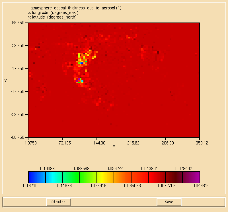
Task 10.5: Calculate aerosol optical depth from the 3D aerosol extinction

TASK 10.5: Using the 3D aerosol extinction, calculate the 0.55 micron aerosol optical depth on the second radiation timestep, and compare this to your AOD from Task 10.2.

Hint
You will need to include contributions from both UKCA and CLASSIC (due to the dust scheme).
Remember to correctly calculate the grid-cell heights.

Python script

To calculate the AOD from the aerosol extinction, you will need to integrate this in the column. To do this you should first multiply by the height of each grid-cell before summing-up.

On ARCHER, an example python script to do this has been provided at /work/n02/n02/ukca/Tutorial/vn10.9/sample_output/Task10.5/calc_AOD.py:

#!/usr/bin/env python

# This file is part of the UKCA Tutorials:
#  http://www.ukca.ac.uk/wiki/index.php/UKCA_Chemistry_and_Aerosol_Tutorials_at_vn10.9

# Copyright (C) 2017  University of Cambridge

# This is free software: you can redistribute it and/or modify it under the
# terms of the GNU Lesser General Public License as published by the Free
# Software Foundation, either version 3 of the License, or (at your option)
# any later version.

# It is distributed in the hope that it will be useful, but WITHOUT ANY
# WARRANTY; without even the implied warranty of MERCHANTABILITY or FITNESS FOR
# A PARTICULAR PURPOSE.  See the GNU Lesser General Public License for more
# details.

# You find a copy of the GNU Lesser General Public License at <http://www.gnu.org/licenses/>.

# Written by N. Luke Abraham 2017-12-11 <nla27@cam.ac.uk> 

# preamble
import iris
import iris.time
import iris.analysis
import numpy as np

fname='/work/n02/n02/ukca/Tutorial/vn10.9/sample_output/Task10.1/atmosa.pa19810901_00'

# constraint on time to get 2nd radiation timestep
tconstr=iris.Constraint(time=lambda cell: cell.point.hour == 2)

# load orography to enable correct calculation of level heights
orog=iris.load_cube(
     '/work/n02/n02/hum/ancil/atmos/n48e/orography/globe30/v1/qrparm.orog',
     iris.AttributeConstraint(STASH='m01s00i033'))

# load all extinction components at 0.55 micron
# must use this way of loading to account for constraint on time
with iris.FUTURE.context(cell_datetime_objects=True):
    ukca=iris.load_cube(fname,[
         iris.Constraint(pseudo_level=3) & iris.AttributeConstraint(STASH='m01s02i530') & tconstr])
    classic=iris.load_cube(fname,[
            iris.Constraint(pseudo_level=3) & iris.AttributeConstraint(STASH='m01s02i540') & tconstr])

# Calculate the correct height of each cell
# add the orography as an auxillary coordinate
auxcoord=iris.coords.AuxCoord(orog.data,standard_name=str(orog.standard_name),long_name="orography",var_name="orog",units=orog.units)
# added in to lat/lon (ht=0,lat=1,lon=2)
ukca.add_aux_coord(auxcoord,(1,2,))
# now calculate the correct altitude above sea-level
factory=iris.aux_factory.HybridHeightFactory(delta=ukca.coord("level_height"),sigma=ukca.coord("sigma"),orography=ukca.coord("surface_altitude"))
# now create the 'altitude' derrived coordinate
ukca.add_aux_factory(factory)
# now calculate the height from the bounds
bounds = ukca.coord('altitude').bounds[:,:,:,1] - ukca.coord('altitude').bounds[:,:,:,0]
    
# mutliply by the height of each cell
ukca.data = ukca.data * bounds
classic.data = classic.data * bounds

# now sum up the column
ukca_int=ukca.collapsed('model_level_number',iris.analysis.SUM)
classic_int=classic.collapsed('model_level_number',iris.analysis.SUM)

# add together
aod=ukca_int.copy()
aod.data = ukca_int.data + classic_int.data
# rename
aod.rename('atmosphere_optical_thickness_due_to_aerosol')

# remove unlimited dimension when writing to netCDF
iris.FUTURE.netcdf_no_unlimited=True

# output to netCDF
iris.save(aod,'Task105_AOD.nc',netcdf_format='NETCDF3_CLASSIC')

On ARCHER, an example python script to calculate the difference from this AOD and the AOD calculated in Task10.2 is also provided at /work/n02/n02/ukca/Tutorial/vn10.9/sample_output/Task10.5/diff_AOD_methods.py:

#!/usr/bin/env python

# This file is part of the UKCA Tutorials:
#  http://www.ukca.ac.uk/wiki/index.php/UKCA_Chemistry_and_Aerosol_Tutorials_at_vn10.9

# Copyright (C) 2017  University of Cambridge

# This is free software: you can redistribute it and/or modify it under the
# terms of the GNU Lesser General Public License as published by the Free
# Software Foundation, either version 3 of the License, or (at your option)
# any later version.

# It is distributed in the hope that it will be useful, but WITHOUT ANY
# WARRANTY; without even the implied warranty of MERCHANTABILITY or FITNESS FOR
# A PARTICULAR PURPOSE.  See the GNU Lesser General Public License for more
# details.

# You find a copy of the GNU Lesser General Public License at <http://www.gnu.org/licenses/>.

# Written by N. Luke Abraham 2017-12-11 <nla27@cam.ac.uk> 

# preamble
import iris

dname='./Task102_AOD.nc'
cname='./Task105_AOD.nc'

diag=iris.load_cube(dname)
calc=iris.load_cube(cname)

# difference the fields
calc.data=calc.data - diag.data

# remove unlimited dimension when writing to netCDF
iris.FUTURE.netcdf_no_unlimited=True

# output to netCDF
iris.save(calc,'Task105_AOD_diff.nc',netcdf_format='NETCDF3_CLASSIC')

Solution to Task 10.5

0.55 micron AOD calculated from the 3D extinction diagnostics.
Difference in AODs calculated by the two methods.

You were asked to

Using the 3D aerosol extinction, calculate the 0.55 micron aerosol optical depth on the second radiation timestep, and compare this to your AOD from Task 10.2.

and were given the hints

You will need to include contributions from both UKCA and CLASSIC (due to the dust scheme).
Remember to correctly calculate the grid-cell heights.

You should use the python script provided to do this.

Note that there will be some small differences between these two fields, especially around coastlines.

Sample output from this task can be found in the /work/n02/n02/ukca/Tutorial/vn10.9/sample_output/Task10.5/ directory on ARCHER, containing the following:

Task105_AOD.nc
Task105_AOD_diff.nc
calc_AOD.py
diff_AOD_methods.py

Task 10.6: Calculate the difference in aerosol impacts when `Sec_Org` is no longer formed from ALICE

TASK 10.6: You should now remove the formation of Sec_Org from the chemical reaction added in Task 6.1, giving

${\textrm {ALICE}}+{\textrm {OH}}\longrightarrow {\textrm {BOB}}$

and assess the impact this has on the aerosol diagnostics calculated in the previous tasks, 10.2, 10.3, and 10.4.

Hint
Remember to remove `Sec_Org` from the diagnostics as well as the reaction.

Note: as this a very short run (that is still spinning-up) and you will only be considering a single timestep, the results will be incredibly noisy.

Required code changes

Modifying a reaction is very similar to adding a new one, although simpler as you are only changing what is already there. The exact routines that will need to be altered will depend on the reaction, but likely include:

`ukca_chem_master.F90`

You must edit the master list of reactions, given by ratb_defs_master for bimolecular reactions, ratt_defs_master for termolecular reactions, rath_defs_master for heterogeneous reactions, or ratj_defs_master for photolysis reactions.

`asad_bimol.F90`, `asad_trimol.F90`, `ukca_hetero_mod.F90`, `asad_hetero.F90`, `ukca_phot2d.F90`, and `ukca_strat_update.F90`

If you added any special code for the reaction(s) to asad_bimol.F90, asad_trimol.F90, ukca_hetero_mod.F90, asad_hetero.F90, ukca_phot2d.F90, or ukca_strat_update.F90 it will need to be altered accordingly. The location of the reaction in the complete list is usually found by searching on the reactants and products, and if these change then the lookup will fail unless it is altered here too.

`asad_flux_dat.F90`

If there are any diagnostics to output the reactions you are modifying, you may need to alter this specification as well if you have changed the reactants and/or products.

Solution to Task 10.6

Difference in AOD.
Difference in single-scattering albedo.
Difference in net downward TOA fluxes.

For a working Rose suite that has completed this task, please see

ARCHER: u-as292@62669
vm: u-as297@62632

The specific Rose changes made are:

ARCHER:

Index: app/fcm_make/rose-app.conf
===================================================================
--- app/fcm_make/rose-app.conf (revision 62651)
+++ app/fcm_make/rose-app.conf (revision 62669)
@@ -42,4 +42,4 @@
 stash_version=1A
 timer_version=3A
 um_rev=vn10.9
-um_sources=branches/dev/lukeabraham/vn10.9_UKCA_Tutorial_Solns@46718
+um_sources=branches/dev/lukeabraham/vn10.9_UKCA_Tutorial_Solns@47380

These differences can be found in the file /home/ukca/Tutorial/vn10.9/worked_solutions/Task10.6/Task10.6_rose.patch on PUMA.

vm:

Index: app/fcm_make/rose-app.conf
===================================================================
--- app/fcm_make/rose-app.conf (revision 62631)
+++ app/fcm_make/rose-app.conf (revision 62632)
@@ -42,4 +42,4 @@
 stash_version=1A
 timer_version=3A
 um_rev=vn10.9
-um_sources=branches/dev/lukeabraham/vn10.9_UKCA_Tutorial_Solns@46718
+um_sources=branches/dev/lukeabraham/vn10.9_UKCA_Tutorial_Solns@47380

The specific UM changes made are:

Index: src/atmosphere/UKCA/asad_flux_dat.F90
===================================================================
--- src/atmosphere/UKCA/asad_flux_dat.F90      (revision 46718)
+++ src/atmosphere/UKCA/asad_flux_dat.F90      (revision 47380)
@@ -1287,9 +1287,9 @@
 
 TYPE(asad_flux_defn), PARAMETER, PUBLIC ::                       &
                                     ukca_tutorial_fluxes(3) = (/ &
-asad_flux_defn('RXN',50134,'B',.FALSE.,0,4,                      &
+asad_flux_defn('RXN',50134,'B',.FALSE.,0,3,                      &
 (/'ALICE     ','OH        '/),                                   &
-(/'BOB       ','Sec_Org   ','          ','          '/)),        &
+(/'BOB       ','          ','          ','          '/)),        &
 asad_flux_defn('DEP',50135,'D',.FALSE.,0,1,                      &
 (/'ALICE     ','          '/),                                   &
 (/'          ','          ','          ','          '/)),        &
Index: src/atmosphere/UKCA/ukca_chem_master.F90
===================================================================
--- src/atmosphere/UKCA/ukca_chem_master.F90   (revision 46718)
+++ src/atmosphere/UKCA/ukca_chem_master.F90   (revision 47380)
@@ -2156,7 +2156,7 @@
 'HCHO      ',1.00e-12,  0.00,    0.00, 1.00, 0.75, 0.25, 2.75, TI,0,0,107),&
 ratb_t1(277,'MACRO2    ','MeOO      ','HO2       ','CO        ','          ',& 
 '          ',1.00e-12,  0.00,    0.00, 1.17, 0.25, 0.00, 0.00, TI,0,0,107),&
-ratb_t1(278,'ALICE     ','OH        ','BOB       ','Sec_Org   ','          ',& 
+ratb_t1(278,'ALICE     ','OH        ','BOB       ','          ','          ',& 
 '          ',2.70E-11,  0.00, -390.00, 0.00, 0.00, 0.00, 0.00, ST,0,0,107) /)
 
 !----------------------------------------------------------------------

These differences can be found in the file /home/ukca/Tutorial/vn10.9/worked_solutions/Task10.6/Task10.6_code.patch on PUMA.

Sample output from this task can be found in the /work/n02/n02/ukca/Tutorial/vn10.9/sample_output/Task10.6/ directory on ARCHER, containing the following:

Task106_AOD.nc
Task106_AOD_diff.nc
Task106_SSA.nc
Task106_SSA_diff.nc
Task106_TOA.nc
Task106_TOA_diff.nc
atmosa.pa19810901_00
diff_AOD_rxn.py
diff_SSA_rxn.py
diff_TOA_rxn.py

Checklist

☐ Output your diagnostics in STASH at: um

\rightarrow

namelist

\rightarrow

Model Input and Output

\rightarrow

STASH Requests and Profiles

\rightarrow

STASH Requests.

☐ When adding new aerosol diagnostics, remember to output on pseudo levels if appropriate.

☐ Make new time and domain profiles as needed.

☐ Run the TidyStashTransform transform macro.

☐ Save your suite.

☐ In the roses/[SUITE-ID] directory, run fcm commit to commit your changes to the repository.: ☐

☐ When modifying chemical reactions, remember to make changes for diagnostics and special cases, as well as altering ukca_chem_master.F90.

☐ The Iris python library can be used to process and visualise Unified Model output.

Tutorial 11

Written by Luke Abraham, Nicolas Bellouin, & Anja Schmidt 2017. With thanks to Ben Johnson.

@@ Line 116: / Line 116: @@
 To make a new domain profile, you should:
-# Right-click anywhere on the list and click the blue plus symbol named '''new section'''
+# Right-click anywhere on the list and click the blue plus symbol ('''<span style="color:blue">+</span>''') named '''new section'''
 #: This will make a new blank line (usually labelled '''1''', the next '''2''' etc.) with a red '''<span style="color: red">X</span>''' next to it.
 # Right-click this new line and click '''View namelist'''.

Difference between revisions of "UKCA Chemistry and Aerosol vn10.9 Tutorial 10"

Revision as of 10:56, 13 December 2017

What you will learn in this Tutorial

Python

Task 10.1: Output aerosol diagnostics

Radiation Timesteps

Making new STASH profiles

Time profiles

Example: Output on Radiation Timesteps

Domain profiles

Example: Output AOT pseudo levels on all model theta levels

Usage profiles

Using your new profiles

Solution to Task 10.1

Task 10.2: Calculate aerosol optical depth

Python script

Solution to Task 10.2

Task 10.3: Calculate the single-scattering albedo

Python script

Solution to Task 10.3

Task 10.4: Calculate the top of the atmosphere net downward radiative flux

Python script

Solution to Task 10.4

Task 10.5: Calculate aerosol optical depth from the 3D aerosol extinction

Python script

Solution to Task 10.5

Task 10.6: Calculate the difference in aerosol impacts when Sec_Org is no longer formed from ALICE

Required code changes

ukca_chem_master.F90

asad_bimol.F90, asad_trimol.F90, ukca_hetero_mod.F90, asad_hetero.F90, ukca_phot2d.F90, and ukca_strat_update.F90

asad_flux_dat.F90

Solution to Task 10.6

Checklist

Task 10.6: Calculate the difference in aerosol impacts when `Sec_Org` is no longer formed from ALICE

`ukca_chem_master.F90`

`asad_bimol.F90`, `asad_trimol.F90`, `ukca_hetero_mod.F90`, `asad_hetero.F90`, `ukca_phot2d.F90`, and `ukca_strat_update.F90`

`asad_flux_dat.F90`