UKCA Chemistry and Aerosol UMvn13.9 Tutorial 16
UKCA Chemistry and Aerosol Tutorials at UMvn13.9
| Difficulty | MEDIUM |
| Time to Complete | 1-2 hours |
| Video instructions | https://www.youtube.com/watch?v=aysibeNdLUY&t=19807s |
What you will learn in this Tutorial
In this tutorial you will learn how to process UKCA data using the VISION toolkit. Further examples of what you can use VISION for can be seen in Russo et al. (2025).
VISION stands for the Virtual Integration of Satellite and In-situ Observation Networks and here we provide examples in how to use the in-situ observations simulator (ISO_simulator) functionality. Satellite functionality is also being developed.
Here you will learn how to run the VISION toolkit and then plot VISION output in a variety of different ways.
Example notebooks are provided, which can be also be viewed here:
and can be found in the
Tutorials/UMvn13.9/notebooks
directory on your virtual machine. Many thanks to Maria Russo for providing these scripts.
You should work through the notebook to see how the plots are generated and become familiar with how to work with the data formats.
At the end of each notebook are some suggested examples which you should think about and complete. If you think of any other visualisation or processing methods, you could also give these a try.
Connect to the notebooks using
NOTE: you may want to close your existing Jupyter lab instance and then restart it via cylc-gui, as this may prevent any issues running high-memory python notebooks. You can either do this via File Shut Down or typing Ctrl-C within the terminal that is running the Cylc GUI server.

References
- Russo, M. R., Bartholomew, S. L., Hassell, D., Mason, A. M., Neininger, E., Perman, A. J., Sproson, D. A. J., Watson-Parris, D., and Abraham, N. L.: Virtual Integration of Satellite and In-situ Observation Networks (VISION) v1.0: In-Situ Observations Simulator (ISO_simulator), Geosci. Model Dev., 18, 181–191, https://doi.org/10.5194/gmd-18-181-2025, 2025.
Data
Here you will compare hourly gridded 3D UKESM ozone to observations made by the BAe-146 research aircraft of the FAAM Airborne Laboritory. These aircraft observations have been made between 2010 and 2020 and have a very high time resolution of 1 second, although they are only defined at a single point in space. In contrast, UKESM has a chemical timestep of 1 hour (i.e. 3600 seconds) and a horizontal resolution of 1.25 x 1.875 degrees (around 100km or so at the equator). VISION is designed to quickly and efficiently co-locate the coarse model data onto the sparse and high-frequency observational data to better enable comparisons and to aid model development and evaluation.
Pre-processed FAAM data has been provided for you along with example UKESM data (a similar dataset can be found here, and this is a very similar model to the ACSIS data from Tutorial 15). We have also provided a small amount of raw model output to allow you to run the toolkit.
Exercise 1: run the VISION toolkit
The VISION toolkit is run on the command line. To do this you will need to find the files within the
Tutorials/UMvn13.9/notebooks/Run_VISION
directory. This contains
cli.py
constants.py
input.json
README
visiontoolkit.py
These files can also be found here:
The README contains some basic instructions. In normal usage you will need to (copy and/or) edit the input.json file to point to the data of interest. This file currently is
{
    "obs-data-path":"/home/vagrant/Tutorials/UMvn13.9/data/Task16/VISION_input/Obs/core_faam_20140704_b860_MAGIC.nc",
    "model-data-path":"/home/vagrant/Tutorials/UMvn13.9/data/Task16/VISION_input/Model/cq626a.pp20140704.pp",
    "orography":"/home/vagrant/Tutorials/UMvn13.9/data/Task16/VISION_input/Obs/orography.pp",
    "chosen-obs-field":false,
    "chosen-model-field":false,
    "outputs-dir":"/home/vagrant/VISION_output/",
    "output-file-name":"ukca_colocated_to_faam_b860.nc"
}
So this will read-in observations from obs-data-path and model data from model-data-path before outputting the co-located file to the file output-file-name located in outputs-dir. You should not need to make any changes to this file.
To be able to run the VISION toolkit, you will first need to activate the conda python environment you are using in a terminal, either using an lxterminal or from within a terminal in Jupyter. First you should get the conda command by
. "/opt/deployment/miniforge/etc/profile.d/conda.sh"
then activate the ukca environment
conda activate ukca
Now you can run the toolkit from within the directory by
python3 visiontoolkit.py --config-file="input.json"
This will produce the following output
.______________________________________________.
|   _     _  _   ______  _  _______  _______   |
|  (_)   (_)| | / _____)| |(_______)(_______)  |
|   _     _ | |( (____  | | _     _  _     _   |
|  | |   | || | \____ \ | || |   | || |   | |  |
|   \ \ / / | | _____) )| || |___| || |   | |  |
|    \___/  |_|(______/ |_| \_____/ |_|   |_|  |
|   _______             _   _      _           |
|  (_______)           | | | |    (_)   _      |
|      _   ___    ___  | | | |  _  _  _| |_    |
|     | | / _ \  / _ \ | | | |_/ )| |(_   _)   |
|     | || |_| || |_| || | |  _ ( | |  | |_    |
|     |_| \___/  \___/  \_)|_| \_)|_|   \__)   |
.______________________________________________.

final_config_namespace is Namespace(verbose=0, config_file='input.json', preprocess_mode_obs=None, preprocess_mode_model=None, orography='/home/vagrant/Tutorials/UMvn13.9/data/Task16/VISION_input/Obs/orography.pp', start_time_override=False, obs_data_path='/home/vagrant/Tutorials/UMvn13.9/data/Task16/VISION_input/Obs/core_faam_20140704_b860_MAGIC.nc', model_data_path='/home/vagrant/Tutorials/UMvn13.9/data/Task16/VISION_input/Model/cq626a.pp20140704.pp', chosen_obs_field=False, chosen_model_field=False, outputs_dir='/home/vagrant/VISION_output/', output_file_name='ukca_colocated_to_faam_b860.nc', history_message='Processed using the NCAS VISION Toolkit to co-locate from model data to the observational data spatio-temporal location.', halo_size=1, spatial_colocation_method='linear', vertical_colocation_coord='air_pressure', source_axes=False, plotname_start='vision_toolkit', plot_mode=0, cfp_cscale='plasma', cfp_mapset_config={}, cfp_input_levs_config={}, cfp_input_general_config={'legend': True, 'markersize': 5, 'linewidth': 0.0, 'title': 'Input: observational field (path, to be used for co-location, with its corresponding data, to be ignored)'}, cfp_input_track_only_config={'legend': True, 'colorbar': False, 'markersize': 0.5, 'linewidth': 0.0, 'title': 'Input: flight track from observational field to co-locate model field onto'}, cfp_output_levs_config={}, cfp_output_general_config={'legend': True, 'markersize': 5, 'linewidth': 0.0, 'title': 'Result: model co-located onto observational path'}, satellite_plugin_config=None, regrid_z_coord=None, regrid_method=None, chosen_obs_fields=None, chosen_model_fields=None, plot_of_input_obs_track_only=False, skip_all_plotting=False, show_plot_of_input_obs=False)
along with information on what the script is doing and how long it is taking. When it has successfully completed the last line should be something like
_____ Time taken (in s) for 'main' to run: 32.9553 _____
When you have finished you may want to deactivate this environment as it may not work with Rose and Cylc commands
conda deactivate
Now you can try plotting the data.
Exercise 2: plot your co-located data

FAAM flight for 4th July 2014.

UKESM data along the flight of 4th July 2014.
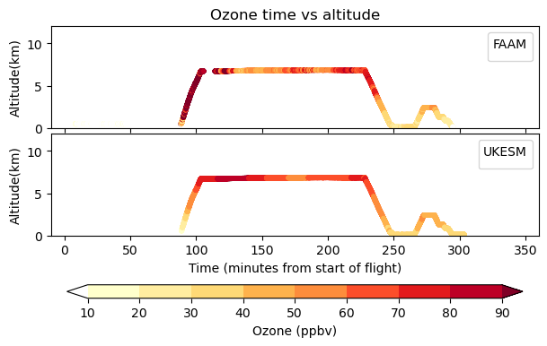
Comparison of FAAM and UKESM data vs altitude.


You should use the VISION_flight.ipynb file:
Nothing should need to be changed, but you should read through the script and try to understand what it is doing at each point.
Exercise 3: Plot plot the full FAAM and co-located UKESM dataset

All FAAM flights 2010-2020

UKESM data along FAAM flights
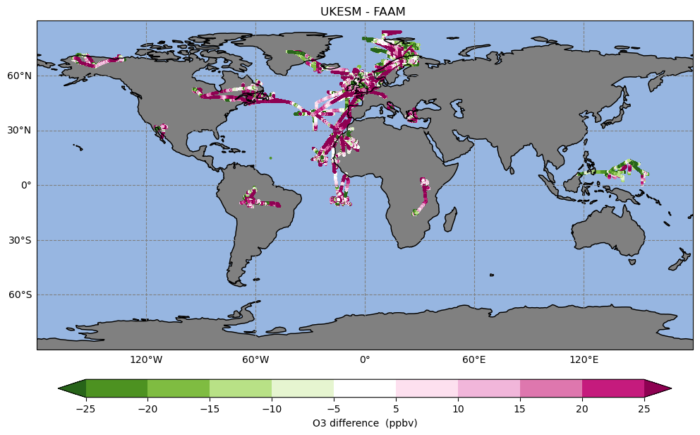
Difference between UKESM and FAAM


While it was quick to co-locate a single flight, it is longer to co-locate many years of data, although using the VISION toolkit is still relatively fast even for this large amount of hourly data. Rather than have you run VISION on the full dataset, we have provided this for you at
/home/ubuntu/Tutorials/UMvn13.9/data/Task16/
in the
FAAM_ozone_cf_compliant_2010_2020/
UKCA_ozone_cf_compliant_2010_2020/
directories. This dataset comprises around 552 separate flights over 471 days across 80 different months.
You should use the VISION_maps.ipynb file:
Note that this notebook will take a long time to run (approx. 20mins or more).
Exercise 4: Plot data only over a selected region

All FAAM flights 2015-2020 in the North Atlantic region
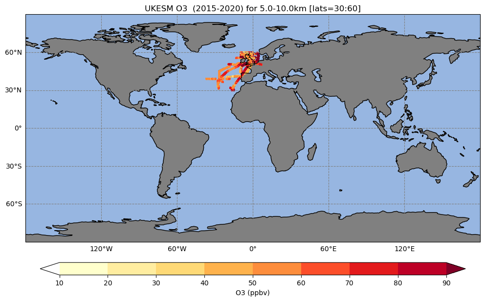
UKESM data along FAAM flights in the North Atlantic region
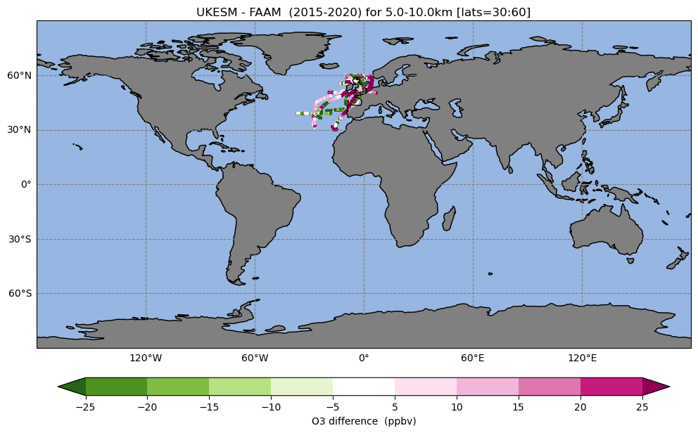
Difference between UKESM and FAAM in the North Atlantic region


In the previous VISION_maps.ipynb file you will have seen the following block of code:
# Select specific start/end year for the analysis (if required)
l_subset_time=False ; start_t='2010-01-01' ; end_t='2020-12-31'
# Select latitudes and altitudes for the analysis (if required).
l_subset_lats= False ; selected_lats= [-30,30]
l_subset_alts= False ; selected_alts=[5000,10000] # units = m
and you can see that all these primary logical are set to False, meaning that these options are not used. Now you should edit this to:
- Only consider flights from 2015 to the end of 2020
- Only consider flights between 30 and 60 degrees latitude
- Only consider flights between 5 and 10km
You should make your changes to this original script. A solution to this exercise can be found in the VISION_region.ipynb file that is in the Solutions/ directory.
| Solution |
|---|
| l_subset_time=True ; start_t='2015-01-01' ; end_t='2020-12-31' |
| l_subset_lats= True ; selected_lats= [30,60] |
| l_subset_alts= True ; selected_alts=[5000,10000] # units = m |
Further exercises
When you have completed this exercise, you should also experiment with plotting different time, region, and altitude ranges.
Exercise 5: Plot histograms of FAAM and UKESM VISION data

Histogram of all FAAM flights, 2010-2020
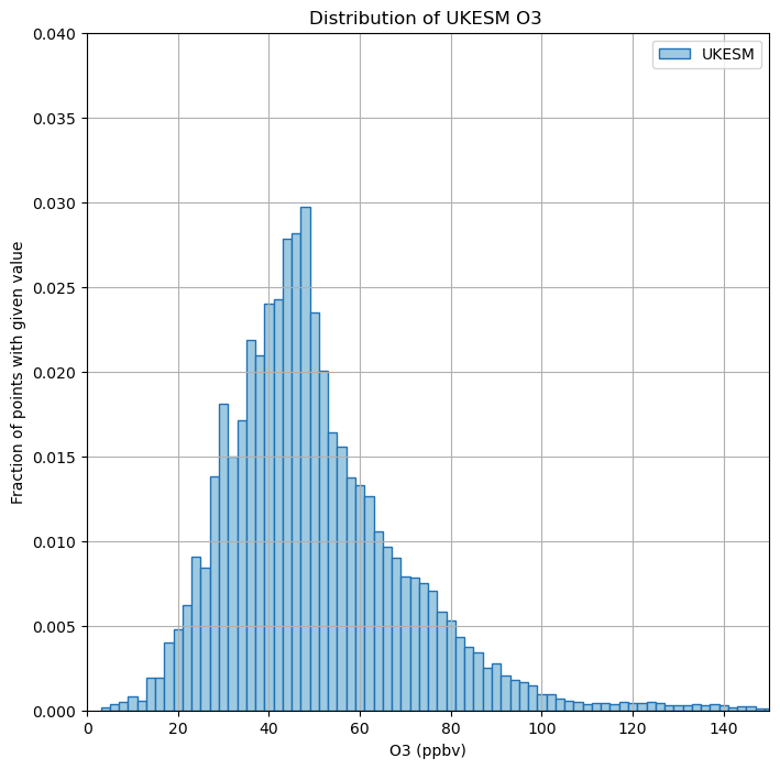
Histogram of UKESM data along FAAM flights
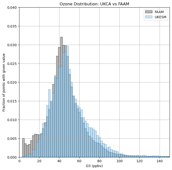
Comparison of both histograms


As well as plotting maps, you can also consider this data in other ways, for example histograms of data comparing e.g. ozone concentration and the number of counts within a specified range. This can be useful to see if the model is able to replicate the ozone distribution as has been observed.
You should use the VISION_histograms.ipynb file:
Further exercises
When you have completed this exercise, you should also experiment with plotting different time, region, and altitude ranges as you did in Exercise 4.
Exercise 6: Plot profiles of FAAM and UKESM VISION data
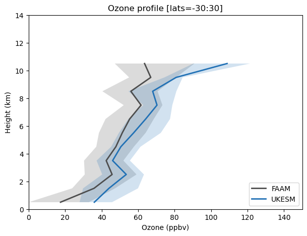
Plot comparing profiles of FAAM flights and corresponding UKESM output for 30S-30N, 2010-2020

You can also plot these data as profiles to see how your model compares against observations in the vertical. This can be done by region and time as was shown earler. For this exercise we shall consider all data in the tropics, 30S-30N.
You should use the VISION_profiles.ipynb file:
Further exercises
When you have completed this exercise, you should also experiment with plotting different time, region, and altitude ranges as you did in Exercise 4.
Checklist
- ☐ Use the VISION toolkit to process model and observational data, and plot these data in a variety of different ways
UKCA Chemistry and Aerosol Tutorials at UMvn13.9
Written by Luke Abraham 2025.