UKCA Chemistry and Aerosol UMvn13.0 Tutorial 13

UKCA Chemistry and Aerosol Tutorials at UMvn13.0

Difficulty	HARD
Time to Complete	2 or more hours
Video instructions

What you will learn in this Tutorial

In this tutorial you will learn how to plot and process UKCA data using the Iris and cf python packages. Example notebooks are provided using both packages, which can be also be viewed here:

• https://github.com/theabro/ukca/tree/master/Tutorials/UMvn13.0/notebooks

and can be found in the

Tutorials/UMvn13.0/notebooks

directory on your virtual machine.

You should work through the notebook to see how the plots are generated. Also compare the different methods between cf and Iris - are some thing easier or harder to do using a particular package. At the end of each notebook are some suggested examples which you should think about and complete.

Observations

This tutorial also makes use of the Bodeker Scientific version 3.4.1 TCO dataset. For ease of use this has been processed from annual files into a single file using the following commands:

for i in `ls *.nc`; do echo $i; ncks -O --mk_rec_dmn time $i $i; done
for i in `ls *.nc`; do echo $i; ncatted -O -a created,global,d,, $i; done
for i in `ls *.nc`; do echo $i; ncatted -O -a units,longitude,o,c,degrees_east $i; done
for i in `ls *.nc`; do echo $i; ncatted -O -a units,latitude,o,c,degrees_north $i; done
ncrcat BSFilledTCO_V3.4.1_????_Monthly.nc ../BSFilledTCO_V3.4.1_Monthly.nc

We would like to thank Bodeker Scientific, funded by the New Zealand Deep South National Science Challenge, for providing the combined NIWA-BS total column ozone database.

Exercise 1: Plot zonal-mean total column ozone

• 

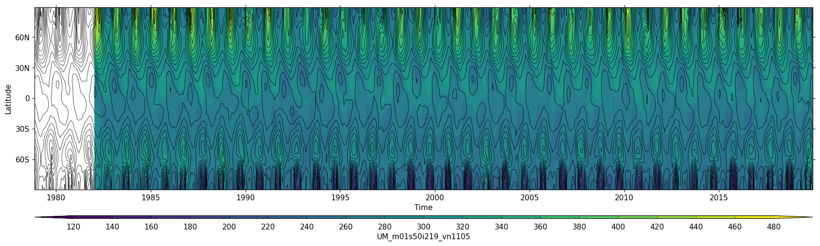
  Total Column Ozone timeseries comparing UKCA and the Bodeker dataset produced using cf-python.

• 

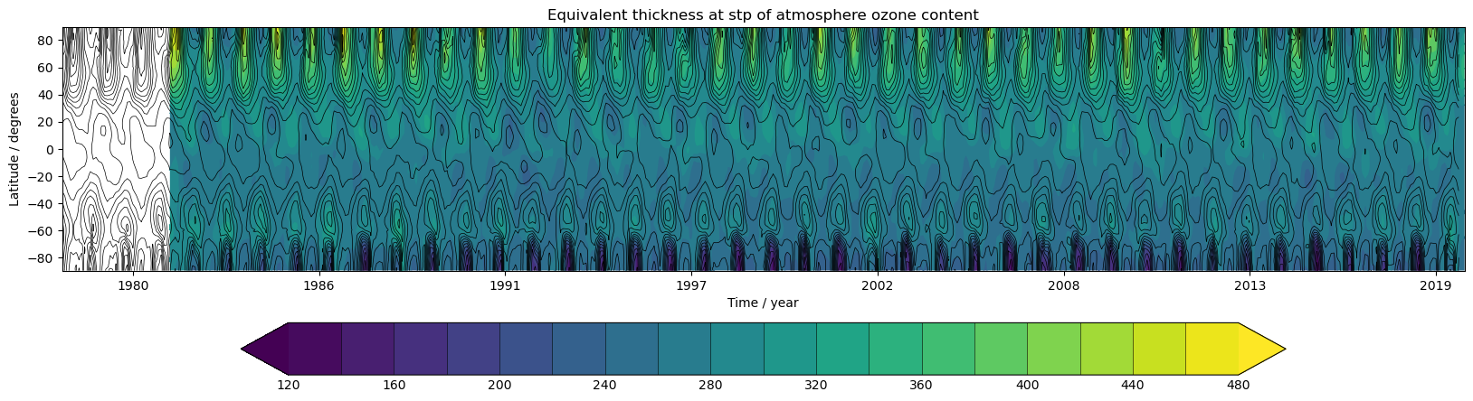
  Total Column Ozone timeseries comparing UKCA and the Bodeker dataset produced using Iris.

Using the *_toz01.ipynb files for cf and for Iris

• cf_toz01.ipynb
• iris_toz01.ipynb

Further exercises

When you have completed this notebook, consider the following exercises to try:

1. Plot members from the CCMI2022 ensemble
2. Produce a plot of the ensemble mean of the 3 ensemble members. How would you go about calculating the ensemble mean?

Exercise 2: Plot the regional time evolution of total column ozone

• 

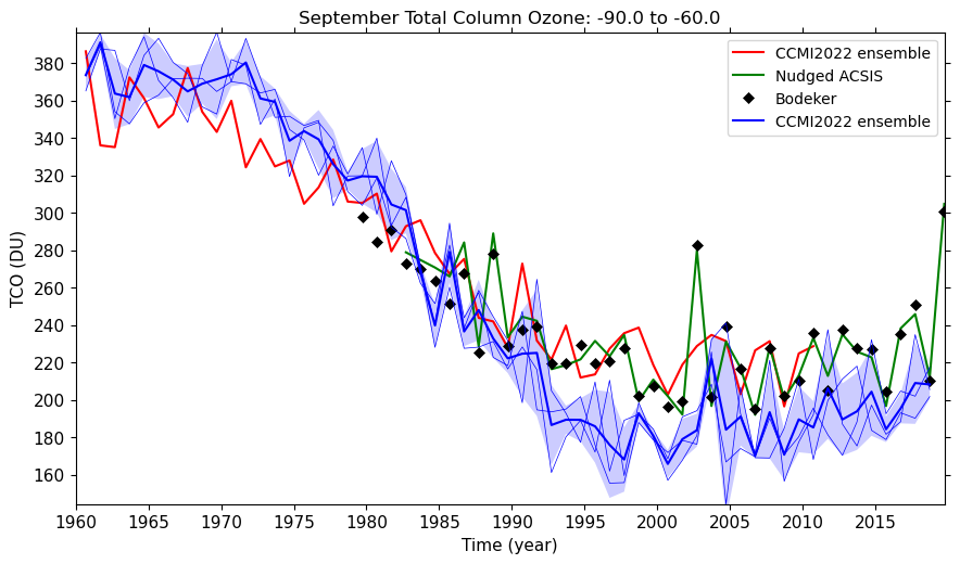
  Total Column Ozone timeseries for September values over the south pole produced using cf-python.

• 

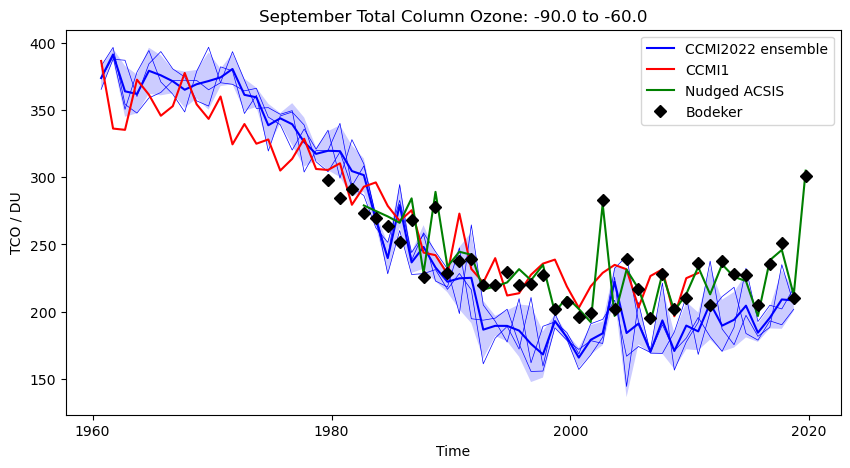
  Total Column Ozone timeseries for September values over the south pole produced using Iris.

Using the *_toz02.ipynb files for cf and for Iris

• cf_toz02.ipynb
• iris_toz02.ipynb

Further exercises

When you have completed this notebook, consider the following exercises to try:

1. Try plotting different months and regions, e.g. March for 60N to 90N
2. Try plotting annual mean TCO from 60S to 60N. How would you go about producing an annual mean of each year?

Hint
Take a look at how to perform statistical collapses in cf.
Take a look at the aggregated_by() method in Iris.

Checklist

☐

UKCA Chemistry and Aerosol Tutorials at UMvn13.0

---

Written by Luke Abraham 2022.