UKCA & UMUI Tutorial 3: Difference between revisions
| Line 66: | Line 66: | ||
There is a rather extensive list of time profiles already existing in this job, and it is possible to add more by making a new one in a blank slot. These time profiles define how the data is time-processed prior to being output. Some profiles, such as '''T6H''' have no meaning, and just output the field as it is every 6 hours, other profiles, such as '''TDAYM''' will result in a daily mean of a field. You can view how these profiles are defined by selecting a profile (it will highlight yellow) and going to '''Profiles → Edit Profile → Edit time''' in the STASH panel menu. |
There is a rather extensive list of time profiles already existing in this job, and it is possible to add more by making a new one in a blank slot. These time profiles define how the data is time-processed prior to being output. Some profiles, such as '''T6H''' have no meaning, and just output the field as it is every 6 hours, other profiles, such as '''TDAYM''' will result in a daily mean of a field. You can view how these profiles are defined by selecting a profile (it will highlight yellow) and going to '''Profiles → Edit Profile → Edit time''' in the STASH panel menu. |
||
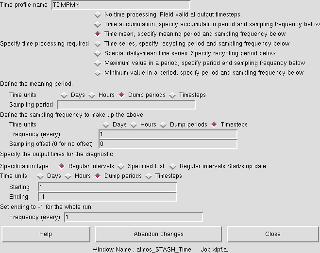
An example of the '''TDMPMN''' time profile is shown in |
An example of the '''TDMPMN''' time profile is shown in Figure 5. This is the climate-meaning time profile, and samples fields every dump period, and should only be used with the '''UPMEAN''' '''usage profile'''. |
||
===Domain Profiles=== |
===Domain Profiles=== |
||
Revision as of 15:02, 28 June 2013
What is STASH?
STASH is the Unified Model's storage handling and diagnostic system. It is designed to cope with the many different configurations that the UM can be used in, but still provide output in a consistent and standard way. A full technical description of STASH can be found in Unified Model Documentation Paper C4 which can be downloaded from the Met Office Collaboration Twiki (password required).
Prognostic and Diagnostic Fields
The UM considers variables (or fields) to be of two different types, prognostic or diagnostic. Prognostic fields are ones which the model must have values for, prior to each timestep, as the equations of motion the model solves require these fields (these are fields such as specific humidity or potential temperature) so they must exist in the model start dump. Diagnostic fields are all other fields that are derrived from prognostic ones, and as such the model does not need to have prior values for these. Ancillary files (such as emissions, SSTs etc) contain prognostic fields.
From a user's perspective, STASH is used to output fields during the run, and from this point of view it does not matter if these are prognostic or diagnostic fields. However, you will need to consider these differences when you add new chemical tracers.
STASH Sections and Items
Each field that is considered by STASH has a unique address which is given by a section and an item number. Prognostic fields are mostly held in section 0 (with the exception of tracers) and diagnostics are organised by areas of the code, e.g. short-wave radiation diagnostics are held in section 1, long-wave radiation diagnostics are held in section 2 etc. Some sections will always be on, and some sections will only be on if a certain process is selected, e.g. the interactive land-surface scheme. Each section can hold up to 512 items, where each item is a separate prognostic or diagnostic field, and can be either 2D or 3D.
Each field has its own entry in a STASHmaster file. There is a master list of fields which is held in the STASHmaster_A file, which is located at
/work/n02/n02/hum/vn8.2/ctldata/STASHmaster/STASHmaster_A
on HECToR, and at
/projects/um1/vn8.2/ctldata/STASHmaster/STASHmaster_A
on MONSooN. This is also a handy list of all the fields that can be outputted from the model, which is easier to search than by going through the UMUI panels. UKCA uses section 34 for chemical tracers and chemical diagnostics, and section 38 for aerosol diagnostics.
Output Files
Before we cover outputting diagnostics from the UMUI STASH panel, we will first cover the different output fields files that are produced by the UM. Output from STASH is sent to different output streams, and there are two types of files used by these streams: standard PP files and climate mean files.
The basic building block of UM output files is a 2D latitude-longitude slice. Surface variables are made up of a single slice, whereas 3D variables are made up of many slices. If you output a 3D varible, such as ozone, this is in fact made up of 85 (as there are 85 model levels) slices.
Standard PP files
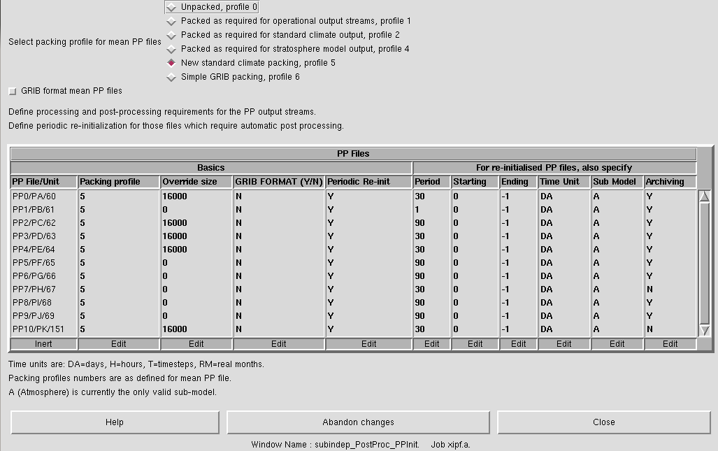
These files are controlled in Model Selection → Post Processing → Initialization and processing of mean and standard PP files. As well as choosing the packing profile (see the Help button for more information) this panel also describes how these different files are treated. As can be seen in Figure 1, there are 11 PP files defined, PP0 to PP10, which correspond to designators pa to pk (with units 60-69, and 151 - these unit numbers may be important in warning and error messages).
The table in this panel can be used to set various properties of these files, such as the time period the file covers, and whether or not the file is archived (i.e. either to the archive/ sub-directory or RDF facility on HECToR, or two the /nerc disk or MOOSE on MONSooN). Being able to change the time period is very useful - while for many simulations monthly mean files are preferred (see the discussion about climate meaning below), often you may wish to output higher frequency data, e.g. 6-hourly. These PP files are usually limited to a finite size and so outputting a month of 6-hourly data may cause the model to crash at run-time. The solution to this is to change how frequently the files are generated, e.g. you could output daily files instead of monthly ones.
The last column in this table controls the archiving of these files. If you have set up your job to archive to a different directory (e.g. to the archive/ sub-direcory on HECToR, or are sending data to the /nerc disk on MONSooN or to the RDF on HECToR, then the files associated with each stream will only be moved if this column is set to Y. If it is N then the file will not be archived but will be deleted if you have requested the Delete superseded PP files in the Model Selection → Post Processing → Main Switch + General Questions panel.
If there is no data being sent to a stream (which is controlled in the STASH panel) then this will automatically be set to N. If you then send data to a stream you will need to manually set it to Y after you have made the diagnostic request.
Climate Mean files
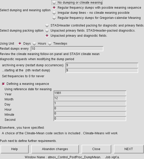
Climate meaning is controlled in the same panel where the restart dump frequency is set: Model Selection → Atmosphere → Control → Post processing, Dumping & Meaning. The main panel is shown in Figure 2. In this example, as is standard for all climate jobs, restart dumps are created every 10 days, and this example as these dumps archived every 9 files, starting with the 9th file after the job is started, i.e. every 3 months (to save space you may choose to change this to 1 year or every 36 files). All other dumps are deleted after they are no longer needed. This means that if the model crashes and needs to be restarted, you will at most have lost 10 days of run. Note: while the model will bit compare on restarting from an old dump, this will not be the case if the dump frequency is changed.
This panel has selected regular frequency dumps with possible meaning sequence so that climate meaning is possible. To do this, you must specify a date for the meaning sequence. Note: you should be careful about this choice of date, especially if you are changing the start-date of the run. It is advised that this meaning squence date is set to be on or before your start date. If it is not you will not generate some of the climate mean files.
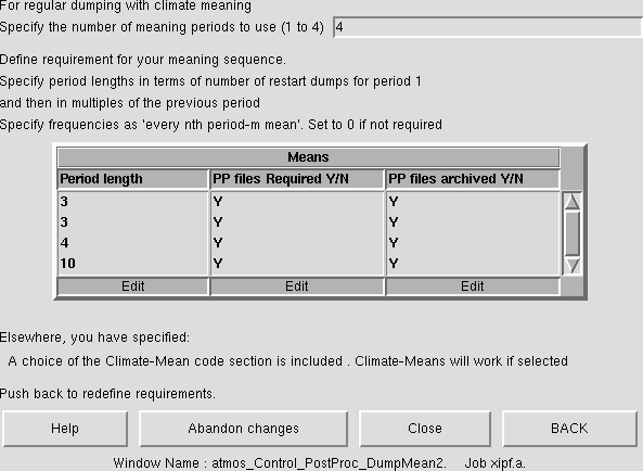
The follow-on window from this panel (shown in Figure 3) gives more details about how climate meaning works. These files work on multiples of the dump period, so the first climate mean file created will be a multiple of 3 dump periods (i.e. 3x10 days, or 30 days. Since we are running a 360-day calendar, this is 1 model month) which is the pm monthly-mean file, which we considered when running existing UKCA Job. The second climate-mean file is a multiple of 3 of the monthly-mean files (i.e. 3x30 days, or 90 days, which is a season), the ps seasonal-mean file (the meaning date is important here to get the correct 3 months for each season). The third climate-mean file is a multiple of 4 of the seasonal-mean files (i.e. 3x90 days, or 360 days, a year), the py annual-mean file. The final file created is a multiple of 10 of the annual-mean files - a decadal-mean px file.
The fields outputted to each of these pm, ps, pa, or px file is the same, and in the same order. All that is different is the meaning done to each field. Note: if you change the dump frequency you will change the frequency of creation of these climate-mean files. In this instance you would need to change the multiple for the first file to get a monthly-mean file correctly.
The UMUI STASH Panel
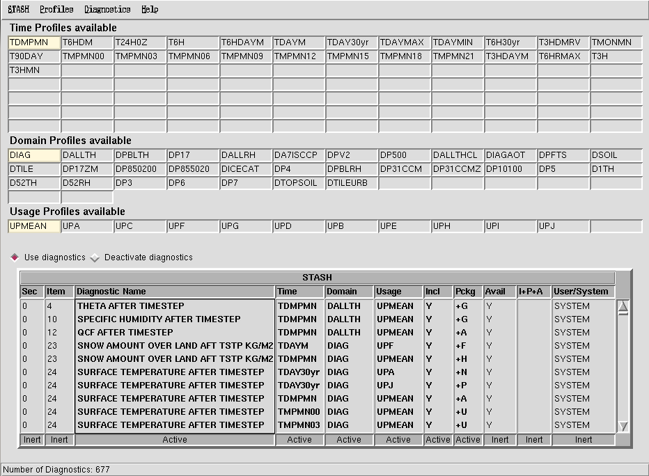
This panel can be found at Model Selection → Atmosphere → STASH → STASH. Specification of Diagnostic requirements and is shown in Figure 4. When you first open this panel you may get a window telling you that system diagnostics have been over-written by user diagnostics - just click continue here. We will cover user diagnostics in the adding new UKCA diagnostics tutorial.
This panel is organised as a table, listing the diagnostics that have been selected (currently - more can be added) and what the time, domain, and usage profile for each diagnostic is. In the table as well as giving the name of each diagnostic, the STASH section and item number is also given, with the table sorted by section, item.
Time Profiles
There is a rather extensive list of time profiles already existing in this job, and it is possible to add more by making a new one in a blank slot. These time profiles define how the data is time-processed prior to being output. Some profiles, such as T6H have no meaning, and just output the field as it is every 6 hours, other profiles, such as TDAYM will result in a daily mean of a field. You can view how these profiles are defined by selecting a profile (it will highlight yellow) and going to Profiles → Edit Profile → Edit time in the STASH panel menu.
An example of the TDMPMN time profile is shown in Figure 5. This is the climate-meaning time profile, and samples fields every dump period, and should only be used with the UPMEAN usage profile.
Domain Profiles
These profiles cover the horizontal and vertical domain covered by fields as they are output. Depending on the diagnostic which is outputted, some of these are on pressure levels, model theta levels, model rho levels, or on a single (e.g. a suface of top of the atmosphere) level etc.. The DALLTH outputs variables on all model theta levels, and it is this domain which UKCA fields (except for surface fields) are usually outputted on. If you edit this profile you can also see that it is possible to output zonal means of fields, or to limit the output to a particular area. This last option can be especially useful if a large amount (e.g. hourly) data is required, but only for a specific part of the world, over the length of a long run.
Usage Profiles
These profiles determine which output stream to use. The UPMEAN profile will send data to the climate-meaning stream discussed above, whereas the UPA profile will send data to the pa file etc.
Note: If you are sending data to the climate-meaning stream UPMEAN you must use the TDMPMN time profile (or a variation thereof), otherwise this output will become corrupted or incorrectly meaned.
The Menu Bar
The STASH panel is unusual for the UMUI in that it has a separate menu bar, rather than using a row of buttons along the bottom of the panel.
STASH
This menu contains the usual Close (i.e. save and close panel) and Abandon (i.e. close without saving) options.
Profiles
As discussed above, you can use the Edit Profile options to view (and change) new or existing profiles. You can also Copy or Delete profiles from this menu.
Diagnostics
This menu contains the items that you will probably use the most. It is here that you can add new diagnostics and change the order of the diagnostics in the table.
Load New Diagnostics (Control-l)
Clicking on this option will bring up a new window, organised by section, listing all the items that can be outputted. This table will list if the field is available in the current model configuration, and there may also be Help available for some diagnostics (if there is, double click where it says "Help").
Remove Diagnostics (Control-r)
You can use this option to remove a diagnostic from the table, although it is easier to type Control-r.
Output Table to File
This outputs the current STASH table, in its current order, to a file (called jobid.A.diags) in your $HOME/umui_jobs directory on PUMA. If you wish to compare the STASH between two jobs it is best to output the STASH table from each and use xxdiff on PUMA, as comparing the two jobs using the UMUI diff is rather confusing when it comes to STASH.
Set Package Switches (Control-t)
You will notice that for some diagnostics in the 8th column of the STASH table (labelled Pckg) there is a letter, e.g. J or +G etc. This corresponds to a package, which is set in this table. This is a useful way of organising diagnostics so that they can be easily turned on or off. For instance, if package J is off then the letter just appears as J (and the I+P+A column would say N), however, this package can be turned on in the package switches table (set to Y), and if it is on this letter now appears as +J. You can only turn diagnostics which are organised through a package on by turning that package on (although you can remove the diagnostic from the package, or add it again but not in package).
Clear Table
Warning: clicking this option will remove all the diagnostics in your STASH table. If you do this in error go to STASH → Abandon to close the STASH window without saving.
Verify Diagnostics (Control-v)
This is a very useful option. When you add new diagnostics you may inadvertantly have made some errors. For some diagnostics you may not be sure what levels (i.e. domain profile) it should be outputted on. For example, UKCA tracer fields should be outputted on model theta levels (DALLTH). If this field is requested on model rho levels (DALLRH) then the Verify Diagnostics window would give
Diag: "O3 MASS MIXING RATIO AFTER TIMESTEP " (34,1) (TDMPMN,DALLRH,UPMEAN)
 DOMAIN PROF ERROR: Use profile on model theta-levels.
Sort Diagnostics
Use this option to order the diagnostics by section, item. When adding new diagnostics they are usually added to the top of the list, rather than in order.
Change Sort Order
This will bring up a box where you can choose which columns are considered (and in which order) when it comes to sorting the diagnostics. The default ordering is equivalent to 1 2 i.e. sort by column 1 (section) then by column 2 (item). I can be very useful to sort by
Help
The Help menu has a more detailed discription of the features and options in the STASH panel.
Task 3.1: add new output
TASK 3.1: Output the instantaneous UKCA ozone field to the ph/UPH stream every 6 hours.
| Hint |
|---|
| You will need to make the changes to the STASH table first, and remember to use Verify Diagnostics. You may then need to change the frequency of output. |
Remember: You will need to delete/move any existing output files in your archive directory.
Written by Luke Abraham 2013
