UKCA Chemistry and Aerosol UMvn13.0 Tutorial 13
UKCA Chemistry and Aerosol Tutorials at UMvn13.0
| Difficulty | HARD |
| Time to Complete | 2 or more hours |
| Video instructions | Walkthrough (YouTube) |
What you will learn in this Tutorial
In this tutorial you will learn how to plot and process UKCA data using the Iris and cf python packages. Example notebooks are provided using both packages, which can be also be viewed here:
and can be found in the
Tutorials/UMvn13.0/notebooks
directory on your virtual machine.
You should work through the notebook to see how the plots are generated. Also compare the different methods between cf and Iris:
- Are some thing easier or harder to do using a particular package?
- Does one package seem to do some things better or worse than the other?
At the end of each notebook are some suggested examples which you should think about and complete. If you think of any other visualisation or processing methods, you could also give these a try.
Connect to the notebooks using
Data
There are a number of different datasets in use in this Tutorial, all of which are Total Column Ozone (TCO). While all the data is gridded, there are a range of resolutions and file types used.
Observations
This tutorial also makes use of the Bodeker Scientific version 3.4.1 TCO dataset. For ease of use this has been processed from annual files into a single file using the following commands:
for i in `ls *.nc`; do echo $i; ncks -O --mk_rec_dmn time $i $i; done
for i in `ls *.nc`; do echo $i; ncatted -O -a created,global,d,, $i; done
for i in `ls *.nc`; do echo $i; ncatted -O -a units,longitude,o,c,degrees_east $i; done
for i in `ls *.nc`; do echo $i; ncatted -O -a units,latitude,o,c,degrees_north $i; done
ncrcat BSFilledTCO_V3.4.1_????_Monthly.nc ../BSFilledTCO_V3.4.1_Monthly.nc
We would like to thank Bodeker Scientific, funded by the New Zealand Deep South National Science Challenge, for providing the combined NIWA-BS total column ozone database.
Model Output
The NERC ACSIS Project
The ACSIS project was a long-term, multi-centre project funded by NERC and as part of this we produced a series UKCA simulations. Model output from one of these simulations is provided in monthly-mean UM "pp" file format. The model configuration is an N96eL85 UKESM1-AMIP (atmosphere-only) configuration at UM version 11.5, where UM winds and temperatures were relaxed to the ERA5 reanalysis dataset. The chemistry scheme used was the Stratosphere-Troposphere scheme that you have been working with in this tutorial. This model simulation used a Gregorian calendar.
Phase 1 of the Chemistry-Climate Model Initiative
UKCA output is submitted to a number of different international model inter-comparison projects, including the first phase of the Chemistry-Climate Model Initiative (CCMI1). Here we submitted data from an atmosphere-only simulation produced using UKCA run at UM version 7.3 at N48L60 resolution used a stratospheric chemistry scheme with explicit treatment of CFCs. Output was processed and converted to CF-standard NetCDF files. As with most UM climate simulations, this model used a 360-day calendar, where each month has 30 days.
Chemistry-Climate Model Initiative 2022
An improved version of UKESM1 was developed which reduced some of the high ozone biases, and was used to perform simulations for the [ https://blogs.reading.ac.uk/ccmi/ccmi-2022/CCMI2022 project]. Here we submitted data from three atmosphere-only UKESM1-AMIP simulations (with to different initial conditions but other settings and forcings the same) run at UM version 11.1 at N96eL85 resolution and uses the improved Stratosphere-Troposphere chemistry and associated settings. Output was processed and converted to CF-standard NetCDF files. As with most UM climate simulations, this model used a 360-day calendar, where each month has 30 days.
Exercise 1: Plot zonal-mean total column ozone
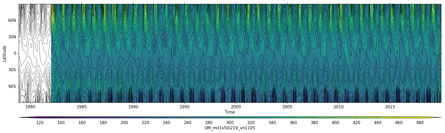
Total Column Ozone timeseries comparing UKCA and the Bodeker dataset produced using cf-python.
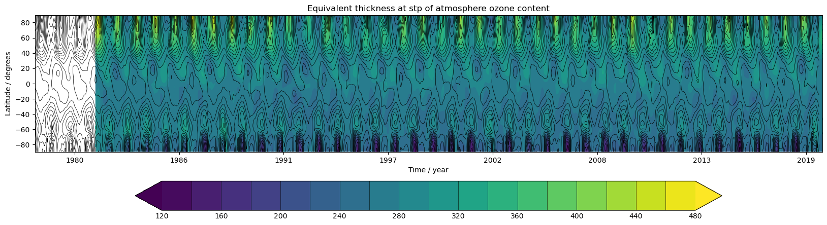
Total Column Ozone timeseries comparing UKCA and the Bodeker dataset produced using Iris.


You should use the *_toz01.ipynb files for cf and for Iris:
Further exercises
When you have completed this notebook, consider the following exercises to try:
- Plot members from the CCMI2022 ensemble
- Produce a plot of the ensemble mean of the 3 ensemble members. How would you go about calculating the ensemble mean?
| Hint |
|---|
| You may need to delete the auxillary coordinates 'forecast_period' and 'forecast_reference_time' in the CCMI2022 ensemble using the cf-python 'f.del_construct()' operation. |
Solutions to these exercises can be found here:
Exercise 2: Plot the regional time evolution of total column ozone
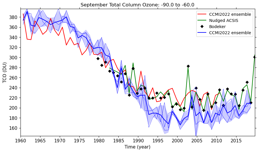
Total Column Ozone timeseries for September values over the south pole produced using cf-python.
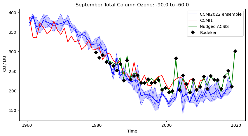
Total Column Ozone timeseries for September values over the south pole produced using Iris.


You should use the *_toz02.ipynb files for cf and for Iris:
Further exercises
When you have completed this notebook, consider the following exercises to try:
- Try plotting different months and regions, e.g. March for 60N to 90N
- Try plotting annual mean TCO from 60S to 60N. How would you go about producing an annual mean of each year?
| Hint |
|---|
| Take a look at how to perform statistical collapses in cf. |
| Take a look at the aggregated_by() method in Iris. |
Solutions to these exercises can be found here:
- March 60N to 90N:
- Annual mean 60S to 60N
Exercise 3: Plot comparisons of total column ozone for specific months
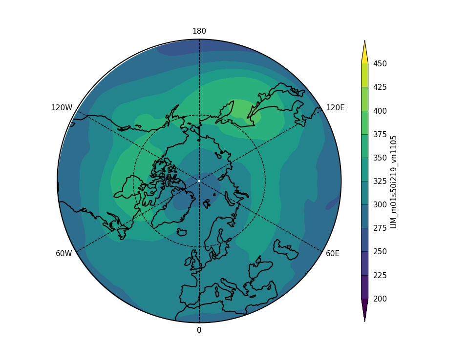
UKCA Total Column Ozone for March 2011 over the north pole produced using cf-python.
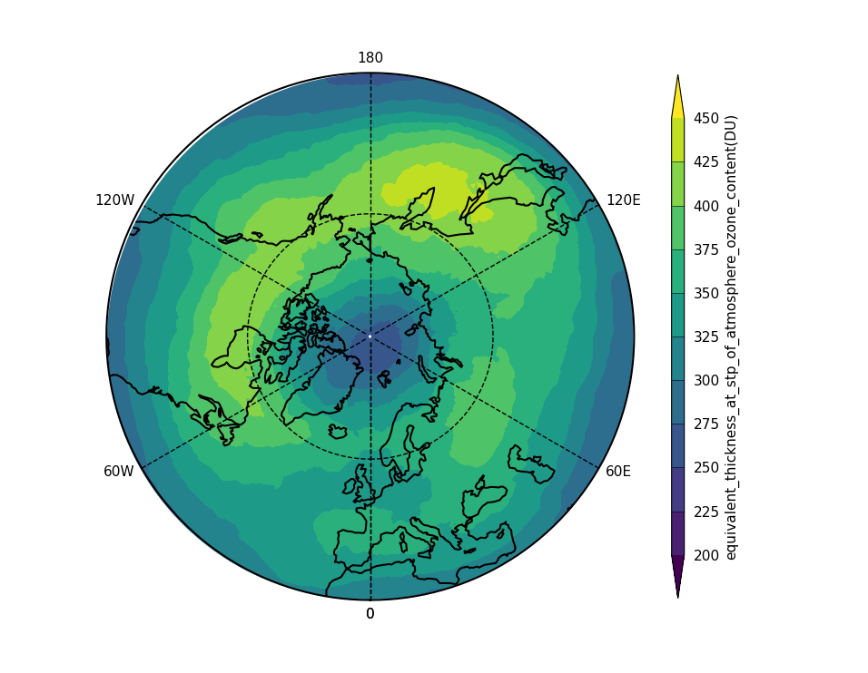
Bodeker Total Column Ozone for March 2011 over the north pole produced using cf-python.
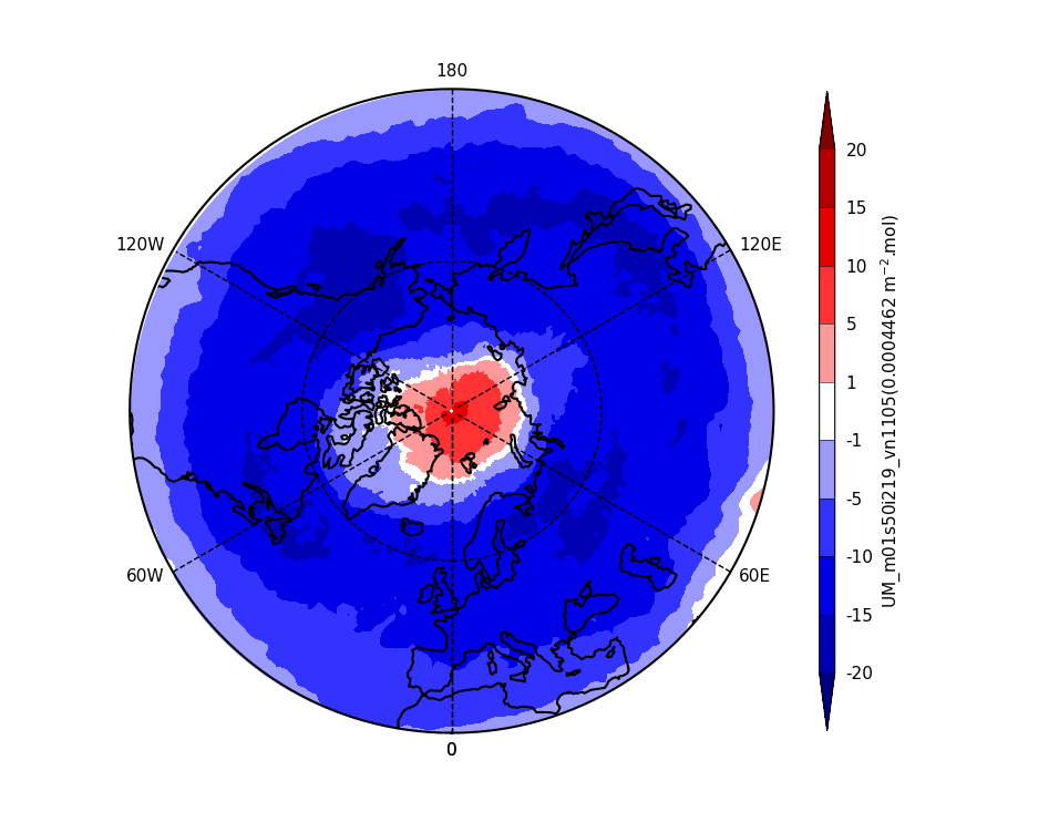
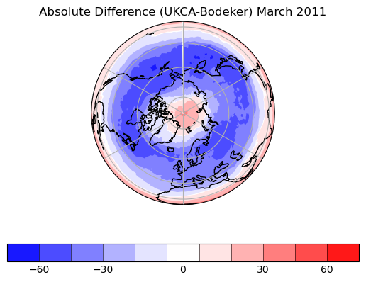
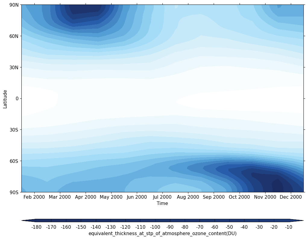
Absolute differences in Total Column Ozone between UKCA and Bodeker for March 2011 over the north pole produced using cf-python.

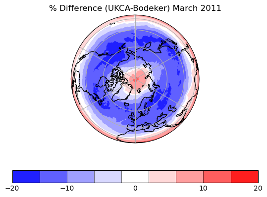
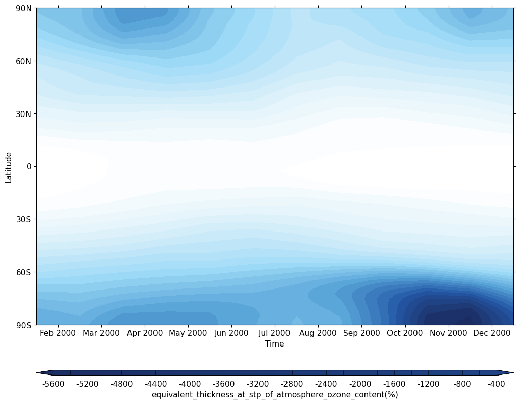
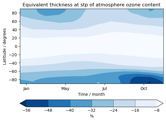
Percentage differences in Total Column Ozone between UKCA and Bodeker for March 2011 over the north pole produced using cf-python.


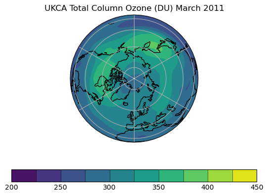
UKCA Total Column Ozone for March 2011 over the north pole produced using Iris.
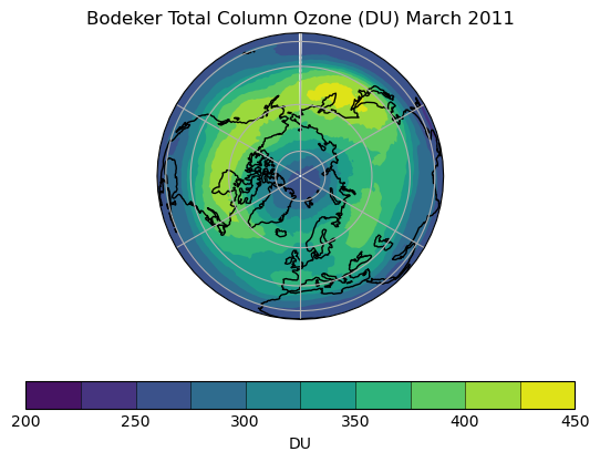
Bodeker Total Column Ozone for March 2011 over the north pole produced using Iris.
Absolute differences in Total Column Ozone between UKCA and Bodeker for March 2011 over the north pole produced using Iris.
Percentage differences in Total Column Ozone between UKCA and Bodeker for March 2011 over the north pole produced using Iris.


You should use the *_toz03.ipynb files for cf and for Iris:
Further exercises
When you have completed this notebook, consider the following exercises to try:
- Try plotting different dates, e.g. September 2002 over the south pole
- How do the CCMI1 and CCMI2022 similations compare. Rather than individual months, try considering decadal climatologies and compare ensemble members.
Solutions to these exercises can be found here:
- September 2002 over the south pole
- CCMI plots
Exercise 4: Plot climatological zonal-mean total column ozone
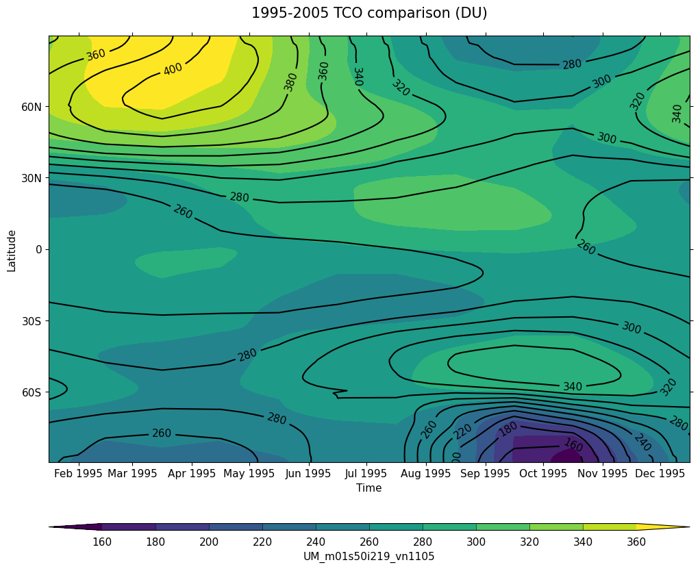
UKCA Total Column Ozone climatology for 1995-2005 produced using cf-python.
Absolute differences in Total Column Ozone for UKCA between 2000-2009 and 1960-1969 produced using cf-python.
Percentage differences in Total Column Ozone for UKCA between 2000-2009 and 1960-1969 produced using cf-python.


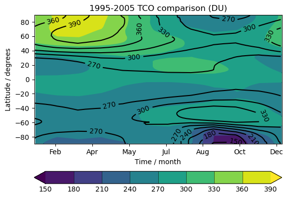
UKCA Total Column Ozone climatology for 1995-2005 produced using Iris.
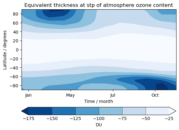
Absolute differences in Total Column Ozone for UKCA between 2000-2009 and 1960-1969 produced using Iris.
Percentage differences in Total Column Ozone for UKCA between 2000-2009 and 1960-1969 produced using Iris.


You should use the *_toz04.ipynb files for cf and for Iris:
Further exercises
When you have completed this notebook, consider the following exercises to try:
- Try comparing the CCMI2022 ensemble members against the ensemble mean.
- Try comparing the nudged UM-UKCA ACSIS data against the CCMI2022 ensemble mean. Here the principal difference between the simulations is the use of nudging to constrain the winds and temperatures.
Solutions to these exercises can be found here:
Further Reading: Processing UKCA Data
You may want to process UKCA data in some way, perhaps to convert to NetCDF for inclusion in a model inter-comparison exercise. For CCMI2022, we processed UKESM1 data from UM pp format to cf-compliant NetCDF using the collection of Iris scripts located at
Due to the time taken to convert the data, which could take several hours, this was done on the JASMIN data analysis platform using the LOTUS batch system.
The work is broken down into 3 main sections:
- The global_attrs.py that sets the necessary global attributes as defined by the MIP data request.
- The convert_pp2nc.py script that does the majority of the work via the main function. This reads-in data from the main JSON tables for the MIP and then uses local JSON tables to define the variables and ensemble members that reference file locations on the JASMIN directory structure.
- Where necessary, data is converted from the model hybrid theta levels to pressure levels using the Fortran program pressureconv.f90 as this is more efficient than doing this regridding in python.
There is also an additional script, cly_bry.py, which specifically considers the creation of the Cly and Bry diagnostic requests. These are quite specific and required the summing of several UKCA tracers.
Take a look through these scripts to see how the data is processed and handled. Take a look at the CCMI2022 ensemble NetCDF files
 Tutorials/UMvn13.0/data/toz_Amon_UKESM1-StratTrop_refD1_r1i1p1f2_gn_19600101-20190101.nc
 Tutorials/UMvn13.0/data/toz_Amon_UKESM1-StratTrop_refD1_r2i1p1f2_gn_19600101-20190101.nc
 Tutorials/UMvn13.0/data/toz_Amon_UKESM1-StratTrop_refD1_r3i1p1f2_gn_19600101-20190101.nc
using the ncdump tool with the -h option to only view the headers to take a look at the files, e.g.
 ubuntu@ip-172-31-34-236:~/Tutorials/UMvn13.0/data$ ncdump -h toz_Amon_UKESM1-StratTrop_refD1_r1i1p1f2_gn_19600101-20190101.nc
 netcdf toz_Amon_UKESM1-StratTrop_refD1_r1i1p1f2_gn_19600101-20190101 {
 dimensions:
 	time = UNLIMITED ; // (708 currently)
 	lat = 144 ;
 	lon = 192 ;
 	bnds = 2 ;
 variables:
 	float toz(time, lat, lon) ;
 		toz:standard_name = "equivalent_thickness_at_stp_of_atmosphere_ozone_content" ;
 		toz:long_name = "Total Column Ozone" ;
 		toz:units = "m" ;
 		toz:um_stash_source = "m01s50i219" ;
 		toz:cell_measures = "area: areacella" ;
 		toz:comment = "Total ozone column calculated at 0 degrees C and 1 bar, such that 1m = 1e5 DU." ;
 		toz:dimensions = "longitude latitude time" ;
 		toz:frequency = "mon" ;
 		toz:modeling_realm = "atmos" ;
 		toz:positive = "" ;
 		toz:type = "real" ;
 		toz:cell_methods = "area: time: mean" ;
 		toz:grid_mapping = "latitude_longitude" ;
 		toz:coordinates = "forecast_period forecast_reference_time level_height model_level_number sigma" ;
 	int latitude_longitude ;
 		latitude_longitude:grid_mapping_name = "latitude_longitude" ;
 		latitude_longitude:longitude_of_prime_meridian = 0. ;
 		latitude_longitude:earth_radius = 6371229. ;
 	double time(time) ;
 		time:axis = "T" ;
 		time:bounds = "time_bnds" ;
 		time:units = "days since 1960-01-01" ;
 		time:standard_name = "time" ;
 		time:long_name = "time" ;
 		time:calendar = "360_day" ;
 		time:stored_direction = "increasing" ;
 	double time_bnds(time, bnds) ;
 	double lat(lat) ;
 		lat:axis = "Y" ;
 		lat:units = "degrees_north" ;
 		lat:standard_name = "latitude" ;
 		lat:long_name = "Latitude" ;
 		lat:stored_direction = "increasing" ;
 	double lon(lon) ;
 		lon:axis = "X" ;
 		lon:units = "degrees_east" ;
 		lon:standard_name = "longitude" ;
 		lon:long_name = "Longitude" ;
 		lon:stored_direction = "increasing" ;
 	double forecast_period(time) ;
 		forecast_period:bounds = "forecast_period_bnds" ;
 		forecast_period:units = "days" ;
 		forecast_period:standard_name = "forecast_period" ;
 	double forecast_period_bnds(time, bnds) ;
 	double forecast_reference_time(time) ;
 		forecast_reference_time:units = "days since 1960-01-01" ;
 		forecast_reference_time:standard_name = "forecast_reference_time" ;
 		forecast_reference_time:calendar = "360_day" ;
 	float level_height ;
 		level_height:bounds = "level_height_bnds" ;
 		level_height:units = "m" ;
 		level_height:long_name = "level_height" ;
 		level_height:positive = "up" ;
 	float level_height_bnds(bnds) ;
 	int model_level_number ;
 		model_level_number:units = "1" ;
 		model_level_number:standard_name = "model_level_number" ;
 		model_level_number:positive = "up" ;
 	float sigma ;
 		sigma:bounds = "sigma_bnds" ;
 		sigma:units = "1" ;
 		sigma:long_name = "sigma" ;
 	float sigma_bnds(bnds) ;

 // global attributes:
 		:activity_id = "CCMI2022" ;
 		:contact = "N. Luke Abraham <n.luke.abraham@ncas.ac.uk>, James Keeble <james.keeble@ncas.ac.uk>" ;
 		:creation_date = "2021-09-24-T17:49:47Z" ;
 		:data_specs_version = "01.00.00" ;
 		:data_version = "20210924" ;
 		:experiment = "Hindcast" ;
 		:experiment_id = "refD1" ;
 		:forcing_index = 2 ;
 		:frequency = "mon" ;
 		:grid = "N96L85 hybrid-theta (1.25 latitude by 1.875 longitude with 85 vertical levels up to 85km)" ;
 		:grid_label = "gn" ;
 		:history = "Model suite-ID(s) = u-cb159, u-cd315. Created using Iris version 2.4.0." ;
 		:initialization_index = 1 ;
 		:institution = "National Centre for Atmospheric Science, Department of Chemistry, University of Cambridge, Lensfield Road, Cambridge, CB2 1EW, UK" ;
 		:institution_id = "NCAS-CAMBRIDGE" ;
 		:license = "CCMI2022 model data produced by NCAS-CAMBRIDGE is licensed under a Creative Commons Attribution-ShareAlike 4.0 International License (https://creativecommons.org/licenses). Consult http://blogs.reading.ac.uk/ccmi/ for terms of use governing CCMI output, including citation requirements and proper acknowledgment. The data producers and data providers make no warranty, either express or implied, including, but not limited to, warranties of merchantability and fitness for a particular purpose. All liabilities arising from the supply of the information (including any liability arising in negligence) are excluded to the fullest extent permitted by law." ;
 		:mip_era = "CMIP6" ;
 		:nominal_resolution = "100 km" ;
 		:physics_index = 1 ;
 		:product = "model-output" ;
 		:realization_index = 1 ;
 		:realm = "atmos" ;
 		:source_id = "UKESM1-StratTrop" ;
 		:source_type = "AER AGCM CHEM" ;
 		:sub_experiment = "none" ;
 		:sub_experiment_id = "none" ;
 		:table_id = "Amon" ;
 		:tracking_id = "d3f54720-e799-4e0e-ab16-ffec9b0b3e2e" ;
 		:variable_id = "toz" ;
 		:variant_label = "r1i1p1f2" ;
 		:Conventions = "CF-1.7" ;
 		:conversion_factor = 1.e-05 ;
 		:in_units = "DU" ;
 		:source = "Data from Met Office Unified Model" ;
 		:um_version = "11.1" ;
 }
Checklist
- ☐ Use cf-python or Iris to process and plot model and observational data
UKCA Chemistry and Aerosol Tutorials at UMvn13.0
Written by Luke Abraham 2022.